

Now, we are actually building a signal processing pipeline that also processes the data! And fortunately, the Datapipeline API has a ready-to-use component for that, too!
In this example, we are going to generate a 32 channel signal with different frequencies per channel. And we are also going to add some random noise to it. Before plotting we are also going to process -- bandpass filtering -- the signal.
import RZ2ephys
from scipy.signal import butter
def example9():
    aSignalGenerator = pipeline.SignalGenerator()
    duration = 1
    frequency = 1.0
    amplitude = 2.0
    theta = 0.0
    sampleRate = 24414
    numChannels = 32
    nyquist = sampleRate/2
    b,a = butter(4,(10/nyquist, 500/nyquist),'bandpass')#make filter coefficients for an 10,500 Hz band pass filter
    filterCoefficients = [b,a]

    aDatasource = pipeline.Datasource()
    aDatasource.setName("Our Signal Datasource")
    aSweepFiltFiltFilterPlugin = pipeline.SweepFiltFiltFilterPlugin()
    aSweepFiltFiltFilterPlugin.setName("Our SweepFiltFiltFilterPlugin")
    aSweepFiltFiltFilterPlugin.setFilterCoeffs(filterCoefficients)
    aDisplay = pipeline.MplSweepDataDisplay(plt)
    aDisplay.setName("Our Signal DataDisplay")
    aDatasink = pipeline.Datasink()
    aDatasink.setName("Our Signal Datasink")

    aDatasource.setOutput(aSweepFiltFiltFilterPlugin)
    aSweepFiltFiltFilterPlugin.setOutput(aDisplay)
    aDisplay.setOutput(aDatasink)

    for n in range(100):
        #generate multichannel data
        time, signalBuffer = aSignalGenerator.makeNChannelSineWave(duration,frequency,amplitude, theta, sampleRate, numChannels)
        lenOfSignal = len(signalBuffer[0:,0])
        sigChunk=np.zeros(lenOfSignal*numChannels)
        sigTupel = tuple(sigChunk)
        #create MCsweep object
        data=RZ2ephys.MCsweep(sigTupel,lenOfSignal,sampleRate,0)
        for chanIdx in range(numChannels):
            data.signal[0:,chanIdx] = (signalBuffer[0:,chanIdx]+np.random.random(lenOfSignal))*np.random.random(1)
        aDataframe = pipeline.Dataframe()
        aDataframe.setFrameNumber(n)
        aDataframe.setData(data)
        aDatasource.addDataframe(aDataframe)
        aDatasource.run()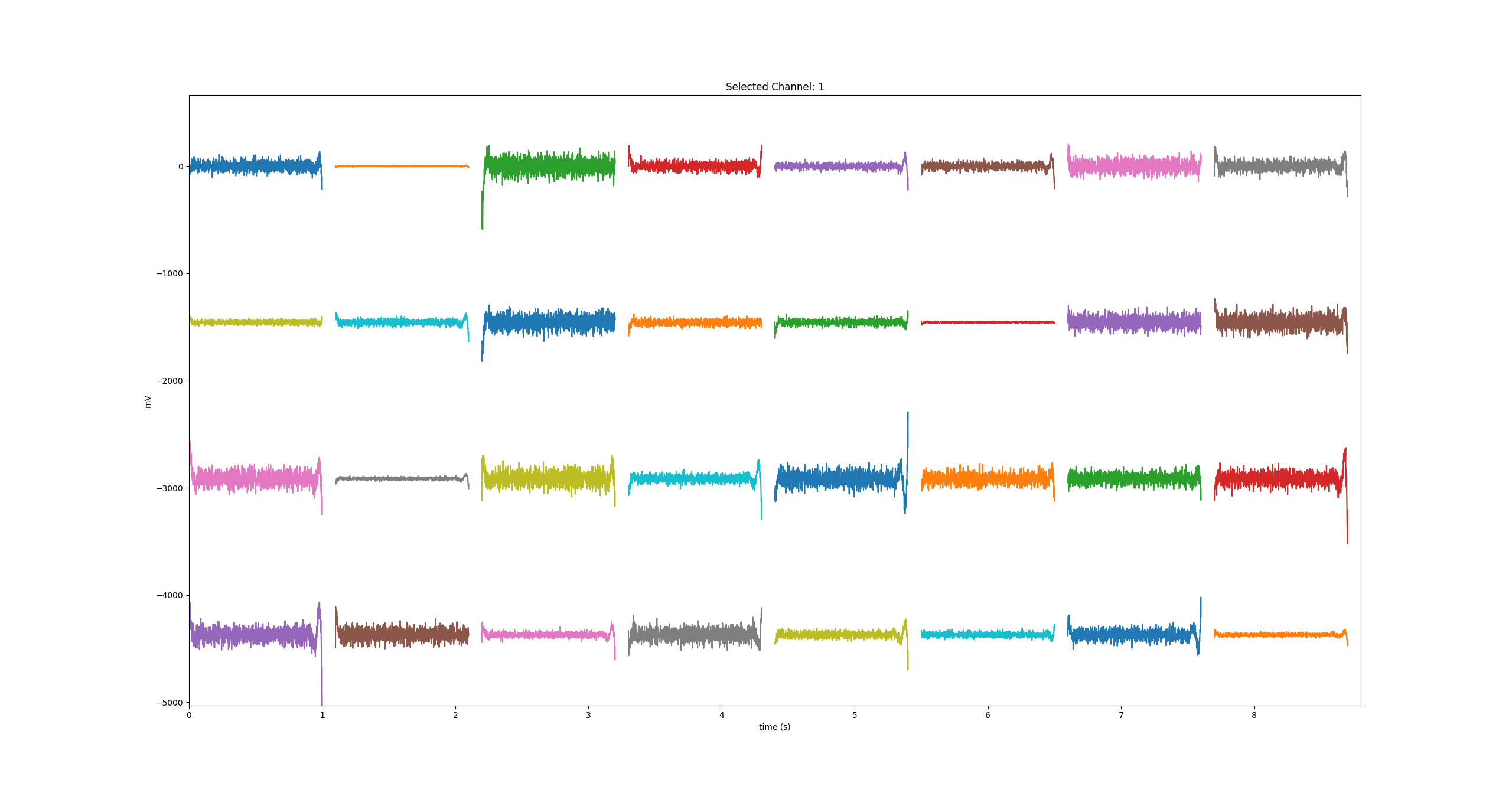
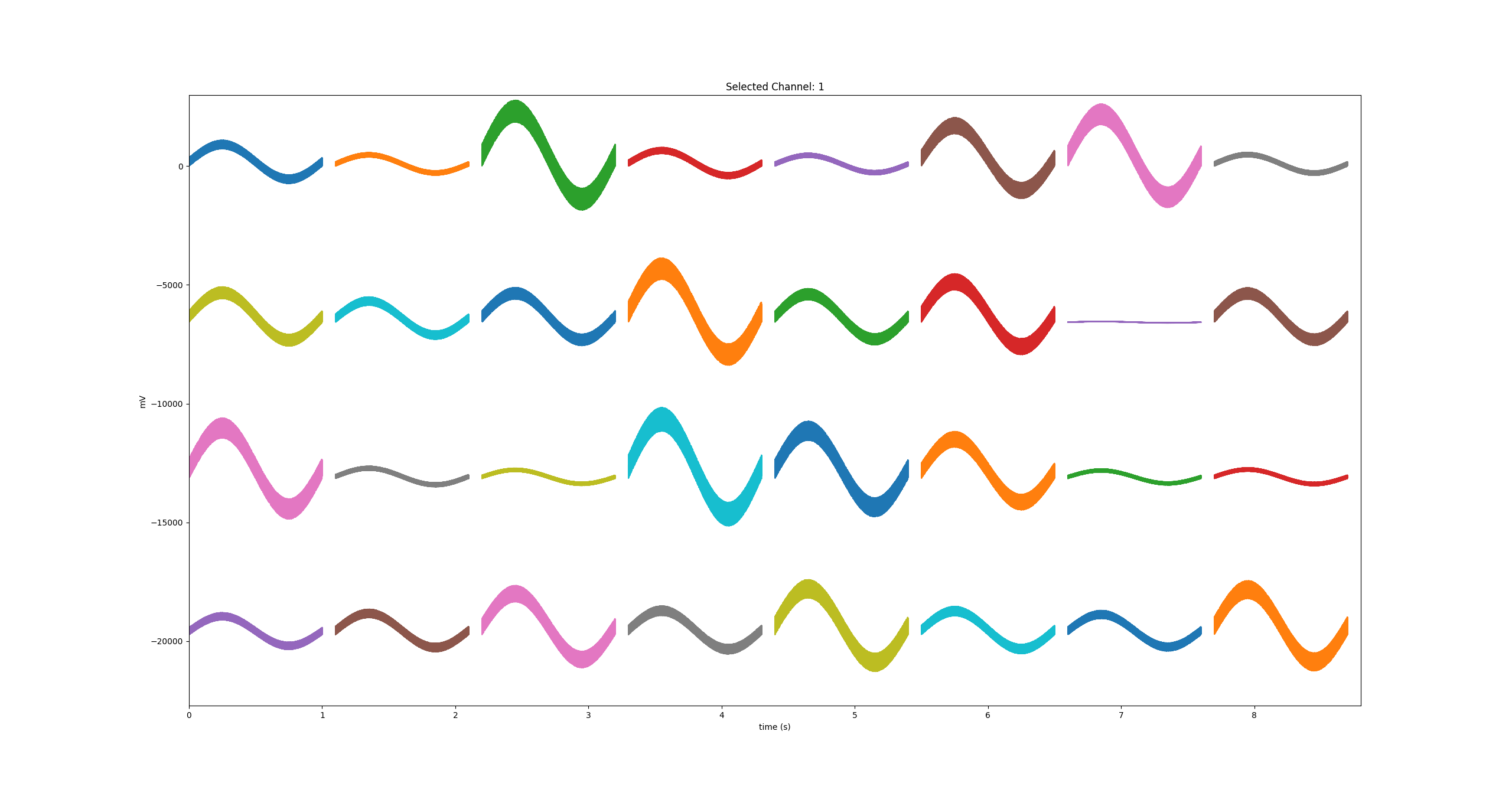
Although the plot looks nice, we cannot see the original signal. Fortunately, we can also plot it. For that, we just have to clone the unfiltered data stream as we have already done it before!
Here is the source code:
import RZ2ephys
from scipy.signal import butter
def example10():
    aSignalGenerator = pipeline.SignalGenerator()
    duration = 1
    frequency = 1.0
    amplitude = 2.0
    theta = 0.0
    sampleRate = 24414
    numChannels = 32
    nyquist = sampleRate/2
    b,a = butter(4,(10/nyquist, 500/nyquist),'bandpass')#make filter coefficients for an 10,500 Hz band pass filter
    filterCoefficients = [b,a]
    numberOfClones = 2

    aDatasource = pipeline.Datasource()
    aCloneDatasource = pipeline.CloneDatasource(numberOfClones)
    aDatasource.setName("Our Signal Datasource")
    aSweepFiltFiltFilterPlugin = pipeline.SweepFiltFiltFilterPlugin()
    aSweepFiltFiltFilterPlugin.setName("Our SweepFiltFiltFilterPlugin")
    aSweepFiltFiltFilterPlugin.setFilterCoeffs(filterCoefficients)
    aDisplay0 = pipeline.MplSweepDataDisplay(plt)
    aDisplay0.setName("Our Signal DataDisplay")
    aDisplay1 = pipeline.MplSweepDataDisplay(plt)
    aDisplay1.setName("Our Signal DataDisplay")

    aDatasource.setOutput(aCloneDatasource)
    aCloneDatasource = pipeline.CloneDatasource(numberOfClones)
    aDatasink0 = pipeline.Datasink()
    aDatasink0.setName("Our Signal Datasink")
    aDatasink1 = pipeline.Datasink()
    aDatasink1.setName("Our Signal Datasink")

    aDatasource.setOutput(aCloneDatasource)
    aCloneDatasource.setOutput(aDisplay0, 0)
    aDisplay0.setOutput(aDatasink0)
    aCloneDatasource.setOutput(aSweepFiltFiltFilterPlugin, 1)
    aSweepFiltFiltFilterPlugin.setOutput(aDisplay1)
    aDisplay1.setOutput(aDatasink1)

    for n in range(100):
        #generate multichannel data
        time, signalBuffer = aSignalGenerator.makeNChannelSineWave(duration,frequency,amplitude, theta, sampleRate, numChannels)
        lenOfSignal = len(signalBuffer[0:,0])
        sigChunk=np.zeros(lenOfSignal*numChannels)
        sigTupel = tuple(sigChunk)
        #create MCsweep object
        data=RZ2ephys.MCsweep(sigTupel,lenOfSignal,sampleRate,0)
        for chanIdx in range(numChannels):
            data.signal[0:,chanIdx] = (signalBuffer[0:,chanIdx]+np.random.random(lenOfSignal))*np.random.random(1)
        aDataframe = pipeline.Dataframe()
        aDataframe.setFrameNumber(n)
        aDataframe.setData(data)
        aDatasource.addDataframe(aDataframe)
        aDatasource.run()
And this is what the output looks like:
It is important to realize that the structure of example 10 is essentially identical to example 5. Let's compare:
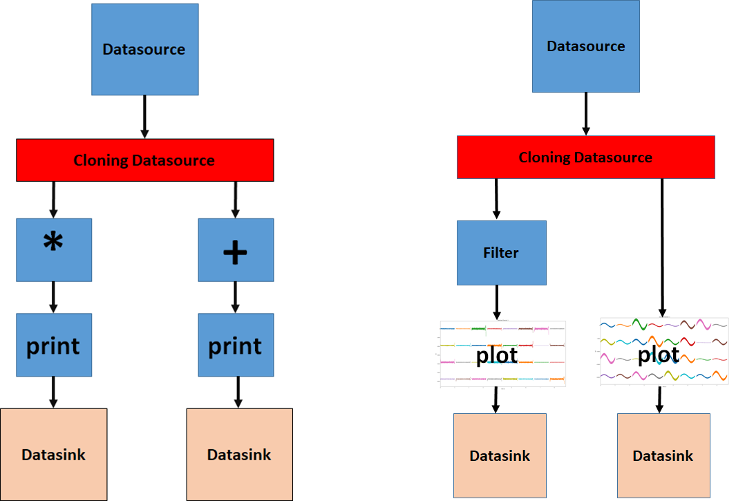
The figure on the right side shows the structure of the pipeline that we have just created in example 10. Conceptually, the structure is very similar to example 5. Instead of creating random numbers, we have created multichannel signals which are then cloned to get two identical data streams. The left branch of the pipeline filters the signals and plots the results and then sends the signals to the datasink. The right branch just plots the signals before sending them to the datasink.