
We know now enough about using the objects of the Datapipline API that we can start to process neurophysiological data.
If you are unfamiliar with the term Neuron, then at least have a look at Wikipedia https://en.wikipedia.org/wiki/Neuron . An excellent read is Kandel and Schwartz Principles Of Neuroscience https://en.wikipedia.org/wiki/Principles_of_Neural_Science
Neurons are electrically excitable cells that are the structural unit of the nervous system. Neurons are able to generate so-called action potentials https://en.wikipedia.org/wiki/Action_potential which are of particular interest in analyzing the response of nervous tissue to certain stimuli. Nervous action potentials are also called spikes, and the process of detecting them is commonly referred to as Spike Detection.
If you are interested in the theory and discovery of spiking neurons, you will not regret reading https://www.izhikevich.org/publications/spikes.htm and https://en.wikipedia.org/wiki/Hodgkin%E2%80%93Huxley_model.
You may also enjoy watching these videos:
Action potential: https://www.youtube.com/watch?v=HYLyhXRp298
Here are two of the greatest achievements in Biology and Neuroscience:
Hubel and Wiesel https://www.youtube.com/watch?v=IOHayh06LJ4 and https://www.youtube.com/watch?v=8VdFf3egwfg
HUBEL DH, WIESEL TN. Receptive fields of single neurons in the cat's striate cortex. J Physiol. 1959;148(3):574-591. doi:10.1113/jphysiol.1959.sp006308
Hodgkin and Huxley: https://www.youtube.com/watch?v=k48jXzFGMc8
HODGKIN AL, HUXLEY AF. A quantitative description of membrane current and its application to conduction and excitation in nerve. J Physiol. 1952;117(4):500-544. doi:10.1113/jphysiol.1952.sp004764
Let's load some sample data:
Source of dataset: A. Sayed Herbawi et al., "CMOS Neural Probe With 1600 Close-Packed Recording Sites and 32 Analog Output Channels," in Journal of Microelectromechanical Systems, vol. 27, no. 6, pp. 1023-1034, Dec. 2018, doi: 10.1109/JMEMS.2018.2872619.
def example11():
from_in_s=1095
to_in_s=1123
sampling_frequency = 5000
#load real data
filteredSignal = np.load("FilteredData.npy")
filteredSignalChunk = filteredSignal[int(from_in_s*sampling_frequency):int(to_in_s*sampling_frequency)]
plt.plot(filteredSignalChunk)
In this example, we don't care about the axis labels o keep the code as minimal as possible. But the y-axis would be the amplitude in micro or millivolt and the x-axis would be the time axis in seconds/milliseconds.
If you run this code, you will get this output:
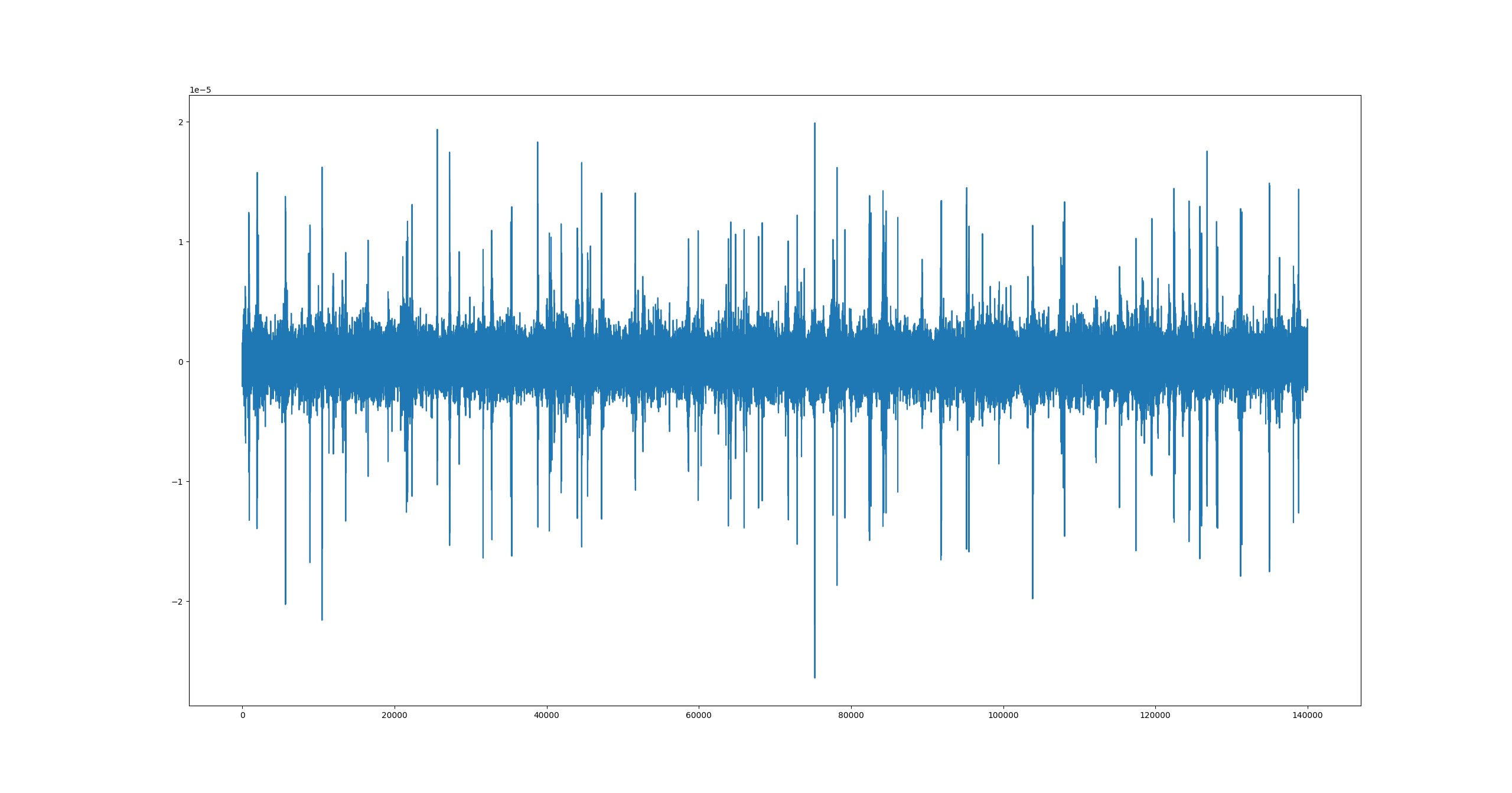
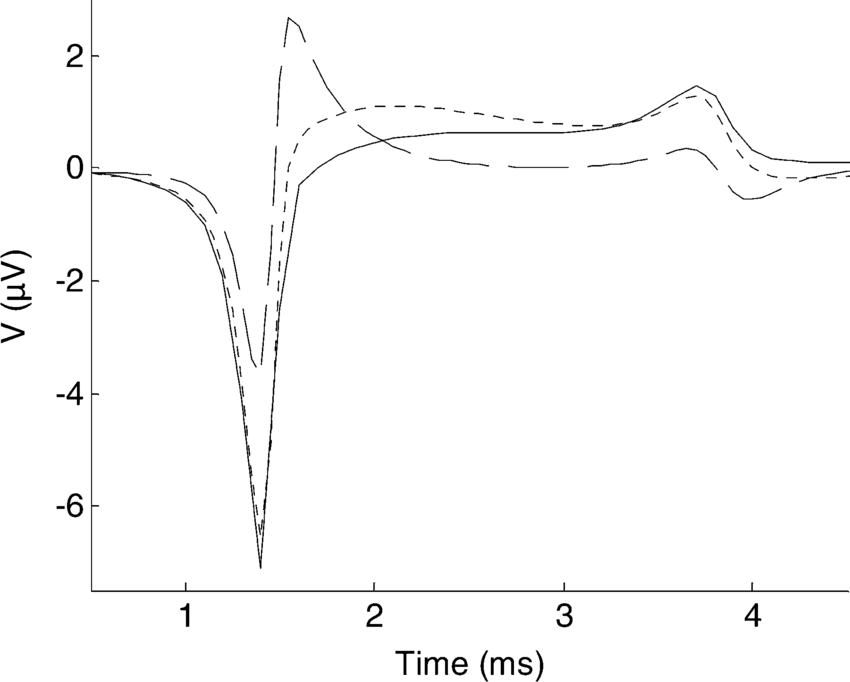
The high-amplitude spiky parts are the recorded action potentials. For the purpose of the part of this tutorial, the signal has already been high-pass filtered and contains frequencies between 300 and 2500 Hz. Feel free to explore the signal by zooming in to different parts of the signal. It will not take long until you discover some action potential -- spike -- resembling the one shown in Figure 15.