

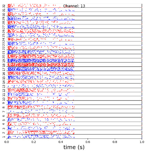
Raster plots are a very informative visualization technique of neural activity. They allow us to easily inspect the neural activity over time span on a single as well as on all channels in a very intuitive way. Furthermore, by taking certain stimulation parameters into account, they also allow us to visualize the spiking activity w.r.t. specific stimuli.
By now it should be no surprise that the Datapipeline API already provides a ready-to-use raster plot plugin. And as you may remember from the very beginning of this tutorial (cf: Fig4 and Fig5), the data stored by the Detector plugin is also stored in special buffers which allow us to store the data of the last N trials or sweeps. And unsurprisingly, those buffers are also already available as plugins which we simply add to our existing pipeline. So now let's get a bit more ambitious and apply all the knowledge we have gained so far and add a single channel as well as multichannel raster plot at the same time.
And here is what we are going to do to make it all happen.
- We need to clone the data stream coming from the spike detector into two streams -- one for the single and one for the multichannel raster plot
- We need to add a buffer containing the data for the 32 channel plot and make it large enough to store the data of 10 sweeps.
- We need also need to add a buffer containing the data for a single channel and make it large enough to store the data of 100 sweeps.
- We need to add the single-channel and the 32 channel raster plot.
- We need to add the display to show the original data
- And we need to add two datasinks to get rid of the data at the end of the pipeline branch.
So let's go and do this!
This what the final code looks like:
def example18():
    sampleRate = 24414
    numChannels = 32
    sweepLen = int(sampleRate/2)
    enableCISimulation = True
    enableBlanking = True
    #set up the stimulation parameter object
    #set stimulation parameters
    level_dB=5  # in dB in relation to 100 uA
    clickRate=50  # 300, 900, 1800
    ears='left' # other options are  'right' and 'both' Must be set to 'left' or 'right' during simulation
    duration = 0.01 # This defines the duration of the  stimulation
    numClicks = 1
    nloop = 0
    reference_Simulation=0.100 # set reference to 100 uA
    levelRePeak = True  # normally we set levels relative to RMS If you want to set them relative to abs max instead, set this to True
    clickShape_CI_Simulation = np.array([0,1,0,-1,0]) # use a biphasic pulse
    blankingEndOffsetInSeconds = 0.02 # This offset shifts the end of the blanking. This can be useful if the filter artifacts occur beyond the actual duration of the stimulation.
    #set up the stimulation parameter object
    stimulatorModule.soundPlayer=stimulatorModule.pygameSoundHardware()
    stimulatorModule.soundPlayer.sampleRate = 25000
    stim=stimulatorModule.clickTrainObject()
    stim.clickShape= clickShape_CI_Simulation
    stim.stimParams['duration (s)']=duration # this parameter controls the duration of the stimulation.
    stim.stimParams['ABL (dB)']=level_dB #ABL means Average Binaural Level
    stim.stimParams['clickRate (Hz)']=clickRate
    stim.stimParams['Nloop']=nloop
    stim.stimParams['numClicks']=numClicks
    stim.reference=reference_Simulation
    stim.clickShape=clickShape_CI_Simulation
    stim.levelRePeak=levelRePeak
    stim.ears=ears
    stim.ready()

    aDatasource = pipeline.Datasource()
    aDatasource.setName("Eyphs PushDataSource")
    sweepSpikeFiltFiltPlugin = pipeline.SweepSpikeFiltFiltPlugin()
    sweepSpikeFiltFiltPlugin.setName("Eyphs SweepSpikeFiltFiltPlugin")

    aSpikeSimulationPlugin = pipeline.SpikeSimulationPlugin()
    aSpikeSimulationPlugin.setName("Eyphs SpikeSimulationPlugin")
    aSpikeSimulationPlugin.loadSpikeTemplates("FilteredSpikeTemplates.npy")
    debugSpikeAmplitudes = [0.0001, 0.0001, 0.0001, 0.0001]
    debugSpikePositions = [0.1, 0.2, 0.3, 0.4]
    aSpikeSimulationPlugin.setDebug(False)
    aSpikeSimulationPlugin.setDebugSpikeAmplitudes(debugSpikeAmplitudes)
    aSpikeSimulationPlugin.setDebugSpikePositions(debugSpikePositions)

    aSweepInterBlankingPlugin = pipeline.SweepInterBlankingPlugin()
    aSweepInterBlankingPlugin.setName("Eyphs SweepInterBlankingPlugin")
    aSweepInterBlankingPlugin.setEndOffsetInSeconds(blankingEndOffsetInSeconds)
    aSweepInterBlankingPlugin.setEnabled(enableBlanking)

    aArtifactSimulationPlugin = pipeline.ArtifactSimulationPlugin()
    aArtifactSimulationPlugin.setName("Eyphs ArtifactSimulationPlugin")
    aArtifactSimulationPlugin.setEnabled(enableCISimulation)
    aSpikeSimulationPlugin = pipeline.SpikeSimulationPlugin()

    aSpikeDetector = pipeline.SpikeDetector()
    aSpikeDetector.setName("Eyphs SpikeDetector")
    aSpikeDetector.setStimEndOffsetInSeconds(blankingEndOffsetInSeconds)

    aCloneDatasource = pipeline.CloneDatasource(2)
    aCloneDatasource.setName("aCloneDatasource")
    aDatasink0 = pipeline.Datasink()
    aDatasink0.setName("Eyphs DataSink0")
    aDatasink1 = pipeline.Datasink()
    aDatasink1.setName("Eyphs DataSink1")

    aNSweepsBufferPlugin = pipeline.NSweepsBufferPlugin()
    aNSweepsBufferPlugin.setName("Eyphs aNSweepsBufferPlugin")

    a100SweepBufferPlugin = pipeline.NSweepsBufferPlugin(numSweeps=100)
    a100SweepBufferPlugin.setName("Eyphs a100SweepsBufferPlugin")

    aNSweepsRasterPlotPlugin = pipeline.NSweepsRasterPlotPlugin()
    aNSweepsRasterPlotPlugin.setName("Ephys aNSweepsRasterPlotPlugin")

    aSingleChannelRasterPlotPlugin = pipeline.NSweepsRasterPlotPlugin(singleChannelPlot = True)
    aSingleChannelRasterPlotPlugin.setName("Ephys aSingleChannelRasterPlotPlugin")

    aDisplay = pipeline.MplSweepDataDisplay(plt)

    #assemble the pipeline
    aDatasource.setOutput(aArtifactSimulationPlugin)
    aArtifactSimulationPlugin.setOutput(sweepSpikeFiltFiltPlugin)
    sweepSpikeFiltFiltPlugin.setOutput(aSpikeSimulationPlugin)
    aSpikeSimulationPlugin.setOutput(aSweepInterBlankingPlugin)
    aSweepInterBlankingPlugin.setOutput(aSpikeDetector)
    aSpikeDetector.setOutput(aCloneDatasource)
    aCloneDatasource.setOutput(aNSweepsBufferPlugin,0)
    aCloneDatasource.setOutput(a100SweepBufferPlugin,1)

    aNSweepsBufferPlugin.setOutput(aNSweepsRasterPlotPlugin)
    aNSweepsRasterPlotPlugin.setOutput(aDisplay)
    aDisplay.setOutput(aDatasink0)

    a100SweepBufferPlugin.setOutput(aSingleChannelRasterPlotPlugin)
    aSingleChannelRasterPlotPlugin.setOutput(aDatasink1)

    for n in range(100):
        #generate multichannel data and random background noise
        sigTupel=tuple(0.000015*np.random.normal(0,1.0, numChannels*sweepLen))
        data=RZ2ephys.MCsweep(sigTupel,sweepLen,sampleRate,0)
        stimObjectCopy = copy.deepcopy(stim)
        aDataframe = pipeline.Dataframe()
        aDataframe.setStimObject(stimObjectCopy)
        aDataframe.setFrameNumber(n)
        aDataframe.setData(data)
        aDatasource.addDataframe(aDataframe)
        aDatasource.run()
And this what the output of the code looks like:
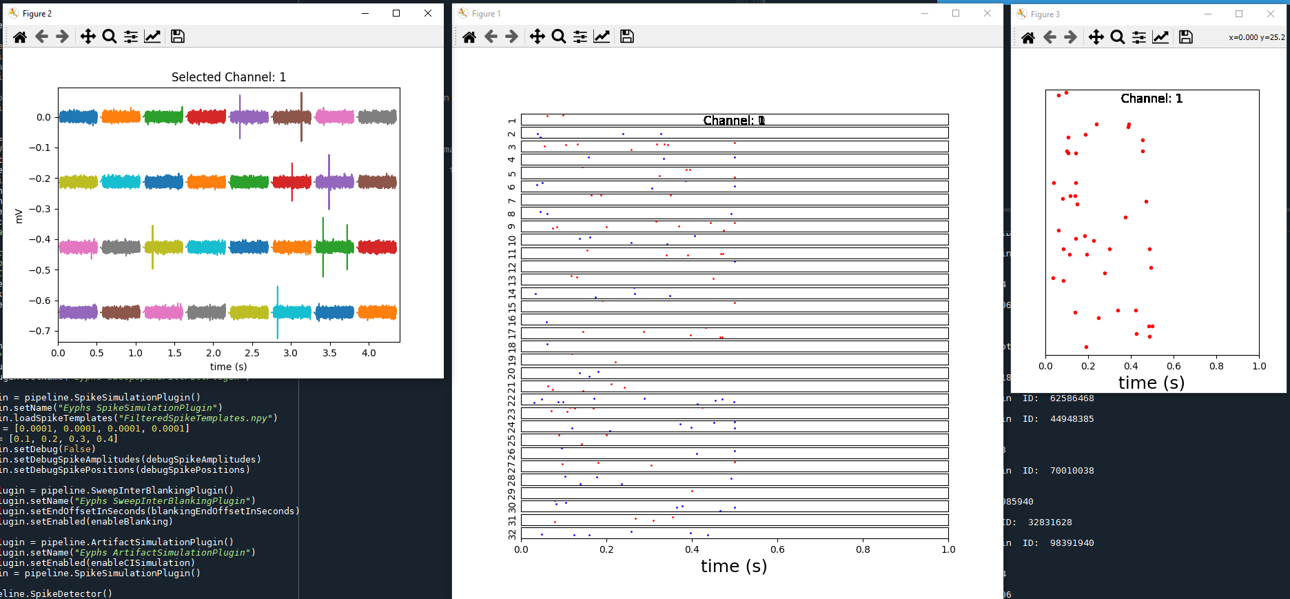
Conceptually, example18() has nothing new to offer. by now you have done it all several times. However, if you look very closely, you may notice that the pipeline has been assembled in a slightly different way compared to what we have done in example17(). And if you compare example18() with what you find in the code of the EphysSearch.py program, you will notice that we have just recreated the simulation pipeline used in that particular program! So congratulations on implementing your first data processing pipeline that can be used to analyze real electrophysiological data!
Tip: If you run this program, you can select the single-channel raster plot of a particular channel by clicking on a channel plot with your mouse.