
Although the median method yields very usable results, it does have its shortcomings. This is explained in [Dolan et al.2009]:
"The background noise signal is made up from the superposition of many signals generated by distinct independent electrical sources and thus can be well-described as broad-band Gaussian noise. A robust estimate of the noise level should be based on statistical properties that
are insensitive to the presence of spikes and artifacts. The median-based method partially meets this requirement. The median of a distribution is more robust to the presence of outliers than measures like the signal standard deviation. An even more robust statistic is
the mode of a distribution (the location of its peak). The mode is very weakly influenced by outliers, regardless of their amplitudes, and only shows a significant bias when the distribution of the outliers substantially overlaps the part of the data distribution around the peak. Unfortunately,
for Gaussian distributed noise the mode equals the mean and therefore conveys no information about the standard deviation of the noise signal. Transforming the Gaussian distribution by taking the absolute value, or other similar rectification transformations also results in
the mode being at 0, so these transformations are of no help in this regard."[Dolan et al.2009]
[Dolan et al.2009] therefore suggest using the envelope of the original signal because its mode is an indicator of the original Gaussian distribution. And for band-limited Gaussian noise, the envelope of the signal is known to follow the Rayleigh distribution. [Papoulis A (1984) ][Proakis JG (1983)]. The probability density function of the resulting Rayleigh distribution is given by:
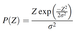
where σ is the standard deviation of the Gaussian noise signal. The Rayleigh distribution is best known for being the distribution of distances from the origin when you have two identical independent Gaussian distributions. For our intents in purposes, the Rayleigh distribution has the very useful property that its mode is exactly equal to the standard deviation of the underlying Gaussian distribution.
The envelope of the original signal can be estimated by using the Hilbert transform.
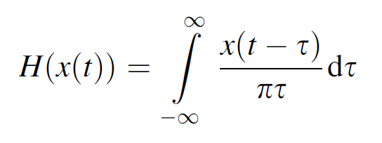
where x(t) is our original signal. Bs using the Hilbert transform we obtain the analytic signal:
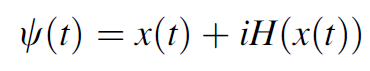
and in polar form:
where A(t) is the instantaneous amplitude of the signal and Θ(t) is the instantaneous phase. This instantaneous amplitude is then taken as an optimal estimate of the envelope of the signal[Fang 1995].
Papoulis A (1984) Probability, random variables, and stochastic processes, 2nd edn. McGraw-Hill, New York
Proakis JG (1983) Digital communications. McGraw-Hill, New York, pp 607–608
[Dolan et al.2009]Dolan K, Martens HC, Schuurman PR, Bour LJ. Automatic noise-level detection for extra-cellular micro-electrode recordings. Med Biol Eng Comput. 2009 Jul;47(7):791-800. doi: 10.1007/s11517-009-0494-4. Epub 2009 May 26. PMID: 19468773.
[Fang 1995]Fang Z-S, Xie N (1995) An analysis of various methods for computing the envelope of a random signal. Appl Ocean Res17:9–19. doi:10.1016/0141-1187(94)00024-H
In Python, the implementation is straight forward:
    #Automatic noise-level detection for extra-cellular micro-electrode recordings
    #Kevin Dolan, H. C. F. Martens, P. R. Schuurman, L. J. Bour
    #Med Biol Eng Comput (2009) 47:791–800
    #DOI 10.1007/s11517-009-0494-4

    def getEnvelopeSTD(self, signal):
        #take the hilbert transform and compute the envelope od the analytic signal
        analytic_signal = hilbert(signal)
        amplitude_envelope = np.abs(analytic_signal)

        #fit the rayleigh distribution to the amplitude envelope of the signal
        x0 = amplitude_envelope
        loc, scale = stats.rayleigh.fit(x0)
        xl = np.linspace(x0.min(), x0.max(), len(signal))
        #get the rayleigh pdf
        rayleigh_pdf = stats.rayleigh(scale=scale, lo
c=loc).pdf(xl)
        modeOfPDF = rayleigh_pdf.max()
        # the mode of the rayleigh pdf is an apprixmation of the standard deviation of the original signal
        indexOfMode = np.where(rayleigh_pdf == modeOfPDF)[0][0]
        envelope_std = xl[indexOfMode]
        return envelope_std
In fact, this is how it is implemented in the Datapipeline API which we are using to build data processing pipelines. The implementation is part of the SpikeProcessing class. Other ways to determine the threshold of the background noise are:
class STDVAlgorithm (Enum):
STD = 0
MAD = 1
ENVELOPE = 2
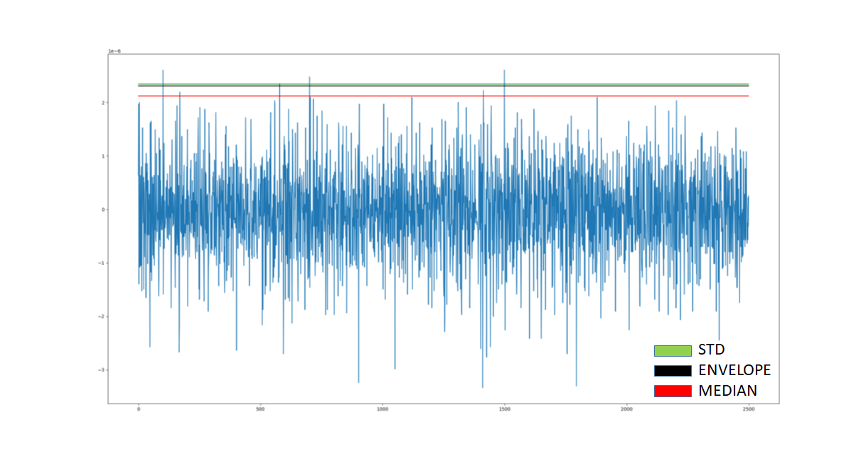
FAST_ENVELOPE = 3where STD is the regular standard deviation, MAD is the median method, the envelope is the method we have just introduced and FAST_ENVELOPE is a substantially faster implementation which makes a systematic error compared to the regular ENVELOPE method but otherwise has no actual drawbacks. In Fig23 we can observe that the median method yields the expected results w.r.t regular standard deviation. And envelope method produces a result that is close to the value of the regular standard deviation because this signal does not have artifacts and its noise level is very low.