6
Auditory Scene
Analysis
- 6.1 What Is Auditory Scene Analysis?
- 6.2 Low- and High-Level Representations of the Auditory Scene: The Case of Masking
- 6.3 Simultaneous Segregation and Grouping
- 6.4 Nonsimultaneous Grouping and Segregation: Streaming
- 6.5 Nonsimultaneous Grouping and Segregation: Change Detection
- 6.6 Summary: Auditory Scene Analysis and Auditory Objects
6.1 What Is Auditory Scene Analysis?
I’m sitting at the
doors leading from the kitchen out into a small back garden. I hear the traffic
in the nearby main road, and the few cars that turn from the main road into the
little alley where the house stands. I hear birds—I can recognize the song of a
blackbird. I hear the rustling of the leaves and branches of the bushes
surrounding the garden. A light rain starts, increasing in intensity. The
raindrops beat on the roofs of the nearby houses and on the windows of the
kitchen.
Sounds help us to know our
environment. We have already discussed, in some detail, the physical cues we
use for that purpose. In previous chapters we discussed the complex processing
required to extract the pitch, the phonemic identity (in case of speech), or
the spatial location of sounds. However, so far we implicitly assumed that the
sounds that need to be processed arise from a single source at any one time. In
real life, we frequently encounter multiple sound sources, which are active
simultaneously or nearly simultaneously. Although the sound waves from these
different sources will arrive at our ears all mixed together, we nevertheless
somehow hear them separately—the birds from the cars from the wind in the
leaves. This, in a nutshell, is auditory scene analysis.
The term “auditory scene analysis”
has been coined by the psychologist Albert Bregman,
and popularized through his highly influential book with that title. In
parallel with the by now classic studies of auditory scene analysis as a
psychoacoustic phenomenon, the field of computational auditory scene analysis
has emerged in recent years, which seeks to create practical, computer-based
implementations of sound source separation algorithms, and feeds back
experience and new insights into the field.
Auditory scene analysis today is
not yet a single, well-defined discipline, but rather a collection of questions
that have to do with hearing in the presence of multiple sound sources. The
basic concept that unifies these questions is the idea that the sounds emitted
by each source reflect its distinct properties, and that it is possible to group those elements of the sounds in time
and frequency that belong to the same source, while segregating those bits that belong to different sources. Sound
elements that have been grouped in this manner are sometimes referred to as an
“auditory stream,” or even as an “auditory object.” If auditory scene analysis
works as it should, one such stream or object would typically correspond to the
sound from a single source. However, “grouping,” “segregation,” “streams,” and “auditory
objects" are not rigorously defined terms, and often tested only
indirectly, so be aware that different researchers in the field may use these
terms to describe a variety of phenomena, and some may even reject the idea
that such things exist at all.
In our survey of auditory scene
analysis, we will therefore reexamine the idea that we group or segregate
sounds, or construct auditory objects under different experimental conditions.
We will start with a very simple situation—a pure tone in a background noise—in
which different descriptions of auditory scene analysis can be discussed in
very concrete settings. Then we will discuss simultaneous segregation—the
ability to “hear out” multiple sounds that occur at the same time, and we will
discuss the way information about the composition of the auditory scene
accumulates with time. Finally, with these issues and pertinent facts fresh in
our minds, we will revisit the issues surrounding the existence and nature of
auditory objects at the end of the chapter.
6.2 Low- and High-Level Representations of the Auditory Scene: The Case of Masking
One of the classical
experiments of psychoacoustics is the measurement of the detection threshold
for a pure-tone “target” in the presence of a white noise “masker.” In these
experiments, the “target” and the “masker” are very different from each
other—pure tones have pitch, while white noise obviously does not.
Introspectively, that special quality of the pure tone jumps out at us. This
may well be the simplest example of auditory scene analysis: There are two
“objects,” the tone and the noise, and as long as the tone is loud enough to
exceed the detection threshold, we hear the tone as distinct from the noise
(Sound Example "Masking a Tone by Noise" on the book's Web site
<flag>). But is this really so?
There is an alternative
explanation of masking that doesn’t invoke the concept of auditory scene
analysis at all. Instead, it is based on concepts guiding decisions based on
noisy data, a field of research often called signal detection theory. The
assumptions that are required to apply the theory are sometimes unnatural,
leading to the use of the term “ideal observer” with respect to calculations
based on this theory. In its simplest form, signal detection theory assumes
that you know the characteristics of the signal to detect (e.g., it is a pure
tone at a frequency of 1,000 Hz) and you know those of the noise (e.g., it is
Gaussian white noise). You are presented with short bits of sounds that consist
either of the noise by itself, or of the tone added to the noise. The problem
you face consists of the fact that noise by nature fluctuates randomly, and may
therefore occasionally slightly resemble, and masquerade as, the pure-tone
target, especially when the target is weak. It is your role as a subject to
distinguish such random fluctuations from the “real” target sound. Signal
detection theory then supplies an optimal test for deciding whether an interval
contains only noise or also a tone, and it even makes it possible to predict
the optimal performance in situations such as a two-interval, two-alternative
forced choice (2I2AFC) experiment, in which one interval consists of noise only
and one interval also contains the tone.
How does this work in the case of
a tone in white noise? We know (see chapter 2) that the ear filters the signal
into different frequency bands, reflected in the activity of auditory nerve
fibers that synapse hair cells at different locations along the basilar
membrane. The frequency bands that are far from the tone frequency would
include only noise. Bands that are close to the tone frequency would include
some of the tone energy and some noise energy. It turns out that the optimal
decision regarding the presence of the tone can be essentially reached by
considering only a single frequency band—the one centered on the tone
frequency. This band would include the highest amount of tone energy relative
to the noise that goes through it. Within that band, the optimal test is
essentially energetic. In a 2I2AFC trial, one simply measures the energy in the
band centered on the target tone frequency during the two sound presentations,
and “detects” the tone in the interval that had the higher energy in that band.
Under standard conditions, no other method gives a better detection rate. In
practice, we can imagine these bands evoking activity in auditory nerve fibers,
and the optimal performance is achieved by simply choosing the interval that
evoked the larger firing rate in the auditory nerve fibers tuned to the signal
frequency.
How often would this optimal
strategy correctly identify the target interval? This depends, obviously, on
the level of the target tone, but performance would also depend in a more subtle
way on the bandwidth of the filters. The reason is that, whereas all the energy
of the tone would always be reflected in the output of the filter that is
centered on the target tone frequency, the amount of noise that would also pass
through this filter would be larger or smaller depending on its bandwidth.
Thus, the narrower the band, the smaller the contribution of the masking noise
to its output, and the more likely the interval with the higher energy would indeed
be the one containing the target tone.
This argument can be reversed: Measure
the threshold of a tone in broadband noise, and you can deduce the width of the
peripheral filter centered at the tone frequency from the threshold. This is
done by running the previous paragraph in the reverse—given the noise and tone
level, the performance of the ideal observer is calculated for different filter
bandwidths, until the calculated performance matches the experimental one. And
indeed, it turns out that tone detection thresholds increase with frequency, as
expected from the increase in bandwidth of auditory nerve fibers. This
argument, originally made by Harvey Fletcher (an engineer in Bell Labs in the first
half of the twentieth century), is central to much of
modern psychoacoustics. The power of this argument stems from the elegant use
it makes of the biology of the early auditory system (peripheral filtering) on
the one hand, and of the optimality of signal detection theory on the other. It
has been refined to a considerable degree by other researchers, leading to the
measurement of the width of the peripheral filters (called “critical bands” in
the literature) and even the shape of the peripheral filters (Unoki et al., 2006). The central finding is that, in many
masking tasks, human performance is comparable to that calculated from theory,
in other words, human performance approaches that of an ideal observer.
However, note that there is no
mention of auditory objects, segregation, grouping, or anything else that is
related to auditory scene analysis. The problem is posed as a statistical
problem—signal in noise—and is solved at a very physical level, by
considerations of energy measurements in the output of the peripheral filters.
So, do we perform auditory scene analysis when detecting pure tones in noise,
or are we merely comparing the output of the peripheral filters, or almost
equivalently, firing rates of auditory nerve fibers?
As we shall see, similar questions
will recur like a leitmotif throughout this chapter. Note that, for the purpose
of signal detection by means of a simple comparison of spike counts, noise and
tone “sensations” would seem to be a superfluous extra, nor is there any
obvious need for segregation or grouping, or other fancy mechanisms. We could
achieve perfect performance in the 2I2AFC test by “listening” only to the
output of the correct peripheral frequency channel. However, this does not mean
that we cannot also perform segregation and grouping, and form separate
perceptual representations of the tone and the noise. Signal detection theory
and auditory scene analysis are not mutually exclusive, but, at least in this
example, it is not clear what added value scene analysis offers.
We encountered similar issues
regarding high-level and low-level representations of sound before: There are
physical cues, such as periodicity, formant frequencies, and interaural level
differences; and then there are perceptual qualities such as pitch, speech
sound identity, and spatial location. We know that we extract the physical cues
(in the sense that we can record neural activity that encodes them), but we do
not perceive the physical cues directly. Rather, our auditory sensations are
based on an integrated representation that takes into account multiple cues,
and that, at least introspectively, is not cast in terms of the physical
cues—we hear pitch rather than periodicity, vowel identity rather than formant
frequencies, and spatial location rather than interaural disparities. In
masking, we face a similar situation: performance is essentially determined by
energy in peripheral bands, but introspectively we perceive the tone and the
noise.
The presence of multiple
representation levels is actually congruent with what we know about the
auditory system. When discussing pitch, speech, and space, we could describe in
substantial details the processing of the relevant parameters by the early
auditory system: periodicity enhancement for pitch, measuring binaural
disparities or estimating notch frequencies for spatial hearing, estimating
formant frequencies of vowels, and so on. On the other hand, the fully
integrated percept is most likely represented in cortex, often beyond the
primary cortical fields.
Can we experimentally dissociate
between low- and high-level representations in a more rigorous way? Merav Ahissar and Shaul Hochstein constructed a conceptual framework, called
reverse hierarchy theory (RHT), to account for similar effects in vision
(Hochstein & Ahissar, 2002). Recently, Nahum, Nelken, and Ahissar (2008)
adapted this framework to the auditory system and demonstrated its validity to
audition as well. RHT posits the presence of multiple representation levels,
and also the fact (which we have emphasized repeatedly) that consciously, we
tend to access the higher representation levels, with their more ecological
representation of the sensory input. Furthermore, RHT also posits that the
connections between different representation levels are dynamic—there are
multiple low-level representations, and under the appropriate conditions we can
select the most informative low-level representation for the current task.
Finding the most informative low-level representation can, however, take a
little while, and may require a search starting at high representation levels
and proceeding backward toward the most informative low-level representations.
Also, this search can find the best low-level representation only if the
stimuli are presented consistently, without any variability except for the
task-relevant one.
Classic psychoacoustic
experiments, where the tone frequency is fixed, provide optimal conditions for
a successful search for the most task-relevant representation, such as the
activity of the auditory nerve fibers whose best frequency matches the
frequency of the target tone. Once the task-relevant representation is
accessed, behavioral performance can reach the theoretical limits set by signal
detection theory. Importantly, if the high-level representation accesses the
most appropriate low-level representation, the two become equivalent and we
then expect a congruence of the conscious, high-level percept with the
low-level, statistically limited ideal observer performance.
This theory predicts that ideal
observer performance can be achieved only under limited conditions. For
example, if the backward search is interrupted, performance will become
suboptimal. Nahum et al. (2008) therefore performed a set of experiments whose
goal was to disrupt the backward search. To do so, they needed a high-level
task that pitted two low-level representations against each other. In chapter 5,
we discussed the detection of tones in noise when the tones are presented to
the two ears in opposite phase (binaural masking level differences, BMLDs). Similar “binaural unmasking” can also be achieved
for other types of stimuli, including speech, if they are presented in opposite
phase to either ear. The improvement in speech intelligibility under these
circumstances is called binaural intelligibility level difference (BILD). Nahum
et al. (2008) therefore used BILD to test the theory.
In the “baseline” condition of
their experiment, Nahum et al. (2008) measured the discrimination thresholds
separately for the case in which words were identical in the two ears (and
therefore there were no binaural disparity cues), and separately for the case
in which words were phase-inverted in one ear (and therefore had the binaural
disparity cues that facilitate detection in noise). The observed thresholds matched
the predictions of ideal observer theory.
The second, crucial part of the
experiment introduced manipulations in aspects of the task that should be
irrelevant from the point of view of ideal observer predictions, but that
nevertheless significantly affected detection thresholds. For example, in one
test condition, trials in which the words were identical in the two ears were
presented intermixed among trials in which the words were phase-inverted in one
ear. This is called “interleaved tracks” in the psychoacoustical
literature. As far as statistical detection theory is concerned, whether
phase-identical and phase-inverted trials are presented in separate blocks or
in interleaved tracks is irrelevant—the theory predicts optimal performance
either way. The results, however, showed a clear difference—the presence of
binaural disparities helped subjects much less in the interleaved tracks than
in the baseline condition, especially when the two words to be distinguished
differed only slightly (by a single phoneme). This is exactly what RHT would
predict. Presumably, the backward search failed to find the optimally
informative lower-level representation because this representation changed from
one trial to the next. Consequently, the optimal task-related representation of
the sounds, which is presumably provided by the activity of the
disparity-sensitive neurons, perhaps in the MSO or the IC, cannot be
efficiently accessed, and performance becomes suboptimal.
What are the implications of this
for auditory scene analysis in masking experiments? RHT suggests that optimal
performance can be achieved only if the conditions in which the experiments are
run allow a successful search for the optimal neural representations. In this
way, it puts in evidence the multiple representation levels of sounds in the
auditory system.
One way of conceptualizing what is
going on is therefore to think of auditory scene analysis as operating at a
high-level representation, using evidence based on neural activity at lower representation
levels. Thus, the auditory scene consists of separate tone and noise objects,
because it presumably reflects the evidence supplied by the peripheral auditory
system: the higher energy in the peripheral band centered on tone frequency.
Both low- and high-level
representations have been studied electrophysiologically
in the context of another masking paradigm, comodulation
masking release (CMR). In CMR experiments, as in BILD, two masking conditions
are contrasted. The first condition is a simple masking task with a noise
masker and a pure tone target. As we already remarked, in this situation ideal
observers, as well as well-trained humans, monitor the extra energy in the
peripheral band centered on the target tone. In the second masking condition,
the masker is “amplitude modulated,” that is, it is multiplied by an envelope
that fluctuates at a slow rate (10–20 Hz). These fluctuations in the amplitude
of the masker produce a “release from masking,” meaning that detecting the
target tone becomes easier, so that tone detection thresholds drop. It is
substantially easier for humans to hear a constant tone embedded in a
fluctuating noise than one embedded in a noise of constant amplitude (Sound
Example "Comodulation Masking Release" on the
book's Web site <flag>).
The curious thing about CMR is
that this drop in threshold is, in a sense, “too large” and depends on the
bandwidth of the noise (figure 6.1). As we discussed earlier,
there is an effective bandwidth, the critical band, around each tone frequency
within which the noise is effective in masking the tone. In regular masking
experiments, adding noise energy outside the critical band has no effect on the
masking. It does not matter whether the noise energy increases if that increase
is outside the critical band because the auditory nerve fibers centered on the
target tone frequency “do not hear” and are not confused by the extra noise. In
contrast, when the masker is amplitude modulated, adding extra noise energy
with the same amplitude modulation outside the critical band does affect
thresholds in a paradoxical way—more noise makes the tone easier to hear. It is
the effect of masker energy away from the frequency of the target tone that
makes CMR interesting to both psychoacousticians and electrophysiologists, because it demonstrates that there is
more to the detection of acoustic signals in noise than filtering by auditory
nerve fibers.
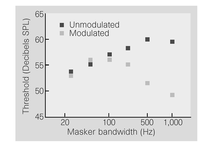
Figure 6.1
The lowest level at
which a tone is detected as a function of the bandwidth of the noiseband that serves as the masker, for modulated and unmodulated noise. Whereas for unmodulated
noise thresholds increase with increases in bandwidth (which causes an increase
in the overall energy of the masker), wide enough modulated maskers are
actually less efficient in masking the tone (so that tones can be detected at
lower levels). This effect is called comodulation
masking release (CMR).
Adapted
from
CMR has neurophysiological
correlates as early as in the cochlear nucleus. Neurons in the cochlear nucleus
often follow the fluctuations of the envelope of the masker, but interestingly,
many neurons reduce their responses when masking energy is added away from the
best frequency, provided the amplitude fluctuations of this extra acoustic
energy follow the same rhythm. In figure 6.2,
two masker conditions are contrasted: one in which the masker is an
amplitude-modulated tone (left), and the other in which additional
off-frequency amplitude-modulated tones are added to it, sharing the same
modulation pattern as the on-frequency masker (right). The response to the
masker is reduced by the addition of comodulated
sidebands (compare the responses at the bottom row, left and right panels).
This makes the responses to tones more salient in the comodulated
condition.
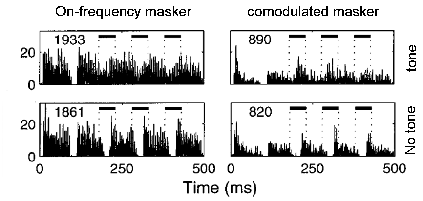
Figure 6.2
Responses of neurons
in the cochlear nucleus to narrowband and wideband modulated maskers (left and
right columns) with and without an added signal (top and bottom rows; here, the
signal consisted of three tone pips in the valleys of the masker). In the comodulated condition, when the masker had larger
bandwidth, the neural responses it evoked were reduced (compare the bottom
panels, left and right). As a result, adding the tone to the wideband masker
results in more salient responses. (Compare the top panels, left and right;
tone presentations are marked by the bars at the top of each panel.)
Adapted
from figure 3 in Pressnitzer et al. (2001).
What causes this reduction in the
responses to the masker when flanking bands are added? Presumably, the
underlying mechanism relies on the activity of “wideband inhibitor” neurons
whose activity is facilitated by increasing the bandwidth of stimuli, which in
turn inhibits other neurons in the cochlear nucleus. Nelken
and Young (1994) suggested the concept of wideband inhibitors to account for
the complex response properties of neurons in the dorsal cochlear nucleus, and
possible candidates have been identified by Winter and
Palmer (1995). A model based on observing the responses of single neurons in
the cochlear nucleus, using the concept of the wideband inhibitor, indeed shows
CMR (Neuert, Verhey, & Winter, 2004; Pressnitzer et al.,
2001).
Thus, just like a human listener,
an ideal observer, observing the responses of cochlear nucleus neurons, could
detect a target tone against the background of a fluctuating masker more easily
if the bandwidth of the masker increases. This picture corresponds pretty much
to the low-level view of tone detection in noise.
Similar experiments have been
performed using intracellular recordings from auditory cortex neurons (Las et
al., 2005), so that changes of the neurons’ membrane potential in response to
the sound stimuli could be observed. As in the cochlear nucleus, a fluctuating
masker evokes responses that follow the envelope of the masker (figure
6.3, bottom, thick black trace). The weak
tone was selected so that it did not evoke much activity by itself (figure
6.3, bottom, thin black trace). When the
two were added together, the locking of the membrane potential to the envelope
of the noise was abolished to a large extent (figure 6.3,
bottom, thick gray trace). The responses to a weak tone in fluctuating noise
can be compared to the responses to a strong tone presented by itself; these
responses tend to be similar (figure 6.3),
especially after the first noise burst following tone onset.
The CMR effect seen in these data is
very pronounced—whereas in the cochlear nucleus, the manipulations of masker
and target cause a quantitative change in the neuronal responses (some
suppression of the responses to the noise as the bandwidth of the masker is
widened; some increase in the responses to the target tone), the effects in
cortex are qualitative: The pattern of changes in membrane potential stops
signaling the presence of a fluctuating noise, and instead is consistent with
the presence of a continuous tone alone.
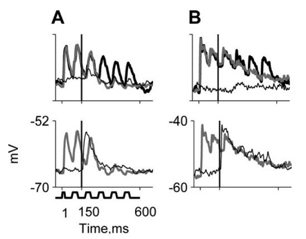
Figure 6.3
The top panels depict
the responses of two neurons (A and B) to noise alone (thick black line; the
modulation pattern is schematically indicated at the bottom of the figure), to
a noise plus tone combination at the minimal tone level tested (gray line; tone
onset is marked by the vertical line), and to a tone at the same tone level
when presented alone (thin black line). The neurons responded to the noise with
envelope locking—their membrane potential followed the on-off pattern of the
noise. Adding a low-level tone, which by itself did not evoke much response,
suppressed this locking substantially. The bottom panels depict the responses
to a tone plus noise at the minimal tone level tested (gray, same as in top
panel) and the response to a suprathreshold level
that saturated the tone response (thin black line). The responses to a
low-level tone in noise and to a high-level tone in silence follow a similar
temporal pattern, at least after the first noise cycle following tone onset.
From figure
6 in Las, Stern, and Nelken (2005).
Originally, the suppression of
envelope locking by low-level tones was suggested as the origin of CMR (Nelken, Rotman, & Bar Yosef, 1999). However, this cannot be the case—if subcortical responses are identical with and without a
tone, then the cortex cannot “see” the tone either. It is a simple matter of neuroanatomy that, for the tone to affect cortical
responses, it must first affect subcortical responses.
As we discussed previously, correlates of CMR at the single-neuron level are already
in the cochlear nucleus. Las et al. (2005) suggested, instead, that neurons
like those whose activity is presented in figure 6.3
encode the tone as separate from the noise—as a separate auditory object.
Presumably, once it has been detected, the tone is fully represented at the
level of auditory cortex in a way that is categorically different from the
representation of the noise.
These experiments offer a glimpse
of the way low-level and high-level representations may operate. At subcortical levels, responses reflect the physical
structure of the sound waveform, and therefore small changes in the stimulus
(e.g., increasing the level of a tone from below to above its masked threshold)
would cause a small (but measureable) change in firing patterns. At higher
levels of the auditory system (here, in primary auditory cortex), the same
small change may result in a disproportionally large change in activity,
because it would signal the detection of the onset of a new auditory object.
Sometimes, small quantitative changes in responses can be interpreted as
categorical changes in the composition of the auditory scene, and the responses
of the neurons in the higher representation levels may encode the results of
such an analysis, rather than merely reflect the physical structure of the
sound spectrum at the eardrum.
6.3 Simultaneous Segregation and Grouping
After this detailed
introduction to the different levels of representation, let us return to the
basics, and specify in more details what we mean by “elements of sounds” for
the purpose of simultaneous grouping and segregation. After all, the tympanic
membrane is put in motion by the pressure variations that are the sum of
everything that produces sound in the environment. To understand the problem
that this superposition of sounds poses, consider that the process that
generates the acoustic mixture is crucially different from the process that
generates a visual mixture of objects. In vision, things that are in front
occlude those that are behind them. This means that occluded background objects
are only partly visible and need to be “completed”; that is, their hidden bits
must be inferred, but the visual images of objects rarely mix. In contrast, the
additive mixing of sound waves is much more akin to the superposition of
transparent layers. Analyzing such scenes brings its own special challenges.
Computationally, the problem of
finding a decomposition of a sound waveform into the sum of waveforms emitted
by multiple sources is ill-posed. From the perspective of the auditory brain,
only the sound waveforms received at each ear are known, and these must be
reconstructed as the sum of unknown waveforms emitted by an unknown number of
sound sources. Mathematically, this is akin to trying to solve equations where
we have only two knowns (the vibration of each eardrum) to determine an a
priori unknown, and possibly quite large, number of unknowns (the vibrations of
each sound source). There is no exact solution for such a problem. The problem
of auditory scene analysis can be tackled only with the help of additional
assumptions about the likely properties of sounds emitted by sound sources in
the real world.
It is customary to start the
consideration of this problem at the level of the auditory nerve representation
(chapter 2). This is a representation of sounds in terms of the variation of
energy in the peripheral, narrow frequency bands. We expect that the frequency
components coming from the same source would have common features—for example,
the components of a periodic sound have a harmonic relationship, and all
frequency components belonging to the same sound source should start at the
same time and possibly end at the same time; frequency components belonging to
the same sound source might grow and decline in level together; and so on and so
forth. If you still recall our description of modes of vibration and impulse
responses from chapter 1, you may appreciate why it is reasonable to expect
that the different frequency components of a natural sound might be linked in
these ways in time and frequency. We will encounter other, possibly more
subtle, grouping cues of this kind later.
The rules that specify how to
select bits of sound that most likely belong together are often referred to as
gestalt rules, in recognition of the importance of gestalt
psychology in framing the issues governing perception of complex shapes. Thus,
common onsets and common amplitude variations are akin to the common fate
grouping principle in vision, according to which elements that move together in
space would be perceived as parts of a single object. The so-called gestalt
rules should be seen as heuristics that work reasonably well in most cases, and
therefore may have been implemented as neural mechanisms.
Let us take a closer look at three
of these grouping cues: common onset, harmonic structure, and common interaural
time difference (ITDs), the latter being, as you may recall from chapter 5, a
cue to the azimuth of a sound source. Whereas the first two turn out to be
rather strong grouping cues, ITDs seem to have a somewhat different role.
6.3.1 Common Onsets
If several frequency
components start at the same time, we are much more likely to perceive them as
belonging to the same auditory object. This can be demonstrated in a number of
ways. We will discuss one such experiment in details here; since it used common
onsets for a number of purposes, it illustrates the level of sophistication of
experiments dealing with auditory scene analysis. It is also interesting
because it pits a high-level and a low-level interpretation of the results
against each other.
Darwin and Sutherland (1984) used
the fine distinction between the vowels /I/ and /e/ in English as a tool for
studying the role of common onsets in auditory perception. These vowels differ
slightly in the frequency of their rather low-frequency first formant (figure
6.4A and Sound Example "Onsets and Vowels
Identity" on the book's Web site <flag>; see also chapter 4 for
background on the structure of vowels). It is possible to measure a formant
boundary—a first formant frequency below which the vowel would generally be
categorized as /I/ and above it as /e/. Since the boundary is somewhat below
500 Hz,
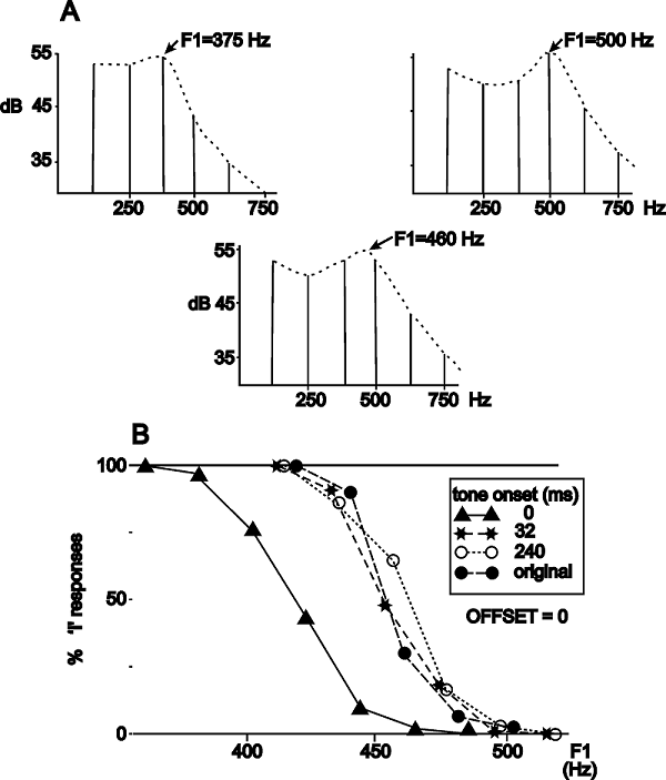
Figure 6.4
(A) Illustration of
the principle of the experiment. The two top spectra illustrate the
first-formant region of the vowels /I/ and /e/ used in the experiment. The
difference between them is in first formant frequency (375 Hz for /I/, 500 Hz
for /e/). At a pitch of 125 Hz, these fall exactly on the third (left) and
fourth (right) harmonics of the fundamental, which are therefore more intense
than their neighbors. When the levels of the two harmonics are approximately
equal, as in the middle spectrum, the first formant frequency is perceived
between the two harmonics (here, at the category boundary between /I/ and /e/).
Thus, by manipulating the relative levels of these two harmonics, it is
possible to pull the perceived vowel between the extremes of /I/ and /e/. (B)
Perceptual judgments for the identity of the vowel (filled circles), for the
vowel with its fourth harmonic increased in level (triangles), and for the
vowel with the fourth harmonic increased in level and starting before the rest
of the vowel (stars and open circles). Onset asynchrony abolished the effect of
the increase in level.
From
figures 1 and 3 in Darwin and Sutherland (1984).
Darwin and Sutherland then
introduced a slight modification of these stimuli. In order to shift the first
formant, they increased the level the fourth harmonic, 500 Hz, of the standard
vowel by a fixed amount. By doing so, the first formant frequency that is
actually perceived is pulled toward higher values, so the sound should be
judged as /e/ more than as /I/. The effect is reasonably large, shifting the
boundary by about 50 Hz (figure 6.4B, triangles;
Sound Example "Onsets and Vowels Identity" <flag>).
The heart of the experiment is a
manipulation whose goal is to reverse this effect. Darwin and Sutherland’s idea
was to reduce the effect of the increase in the level of the fourth harmonic by
supplying hints that it is not really part of the vowel. To do that, they
changed its onset and offset times, starting it before or ending it after all
the other harmonics composing the vowel. Thus, when the fourth harmonic started
240 ms earlier than the rest, subjects essentially disregarded its high level when
they judged the identity of the vowel (figure 6.4B,
circles and stars; Sound Example "Onsets and Vowels Identity"
<flag>). A similar, although smaller, perceptual effect occurred with
offsets.
These results lend themselves very
naturally to an interpretation in terms of scene analysis: Somewhere in the
brain, the times and levels of the harmonics are registered. Note that these
harmonics are resolved (chapters 2 and 3), as they are far enough from each
other to excite different auditory nerve fibers. Thus, each harmonic excites a
different set of auditory nerve fibers, and a process that uses common onset as
a heuristic observes this neural representation of the spectrotemporal
pattern. Since the fourth harmonic started earlier than the rest of the vowel,
this process segregates the sounds into two components: a pure tone at the
frequency of the fourth harmonic, and the vowel. As a result, the energy at 500
Hz has to be divided between the pure tone and the vowel. Only a part of it is
attributed to fourth harmonic of the vowel, and the vowel is therefore
perceived as more /I/-like, causing the reversal of the shift in the vowel
boundary.
However, there is another possible
interpretation of the same result. When the 500-Hz tone starts before the other
harmonics, the neurons responding to it (the auditory nerve fibers as well as
the majority of higher-order neurons throughout the auditory system) would be
activated before those responding to other frequencies, and would have
experienced spike rate adaptation. Consequently, their firing rates would have
declined by the time the vowel started and the other harmonics came in. At the
moment of vowel onset, the pattern of activity across frequency would therefore
be consistent with a lower-level fourth harmonic, pulling the perception back
toward /I/. We have here a situation similar to that discussed earlier in the
context of masking—both high-level accounts in terms of scene
analysis or low-level accounts in terms of subcortical
neural firing patterns can be put forward to explain the results. Is it
possible to falsify the low-level account?
Darwin and Sutherland (1984) tried
to do this by adding yet another element to the game. They reasoned that, if
the effect of onset asynchrony is due to perceptual grouping and segregation, they
should be able to reduce the effect of an asynchronous onset by “capturing” it
into yet another group, and they could then try to signal to the auditory
system that this third group actually ends before the beginning of the vowel.
They did this by using another grouping cue: harmonicity.
Thus, they added a “captor tone” at 1,000 Hz, which started together with the
500 Hz tone before vowel onset, and ended just at vowel onset. They reasoned
that the 500 Hz and the 1,000 Hz would be grouped by virtue of their common
onset and their harmonic relationship. Ending the 1,000 Hz at vowel onset would
then imply that this composite object, that is, both the 1,000- and the 500-Hz
component, disappeared from the scene. Any 500-Hz sound energy remaining should
then be attributed to, and grouped perceptually with, the vowel that started at
the same time that the captor ended, and the 500-Hz component should exert its
full influence on the vowel identity. Indeed, the captor tone reversed, at
least to some degree, the effect of onset asynchrony (Sound Example "Onsets
and Vowels Identity" <flag>). This indicates that more must be going
on than merely spike rate adaptation at the level of the auditory nerve, since
the presence or absence of the 1,000-Hz captor tone has no effect on the
adaptation of 500-Hz nerve fibers.
The story doesn’t end here, however,
since we know today substantially more than in 1984 about the sophisticated
processing that occurs in early stages of the auditory system. For example, we
already encountered the wideband inhibition in the cochlear nucleus in our
discussion of CMR. Wideband inhibitor neurons respond poorly to pure tones, but
they are strongly facilitated by multiple tones, or sounds with a wide
bandwidth. They are believed to send widespread inhibitory connections to most
parts of the cochlear nucleus.
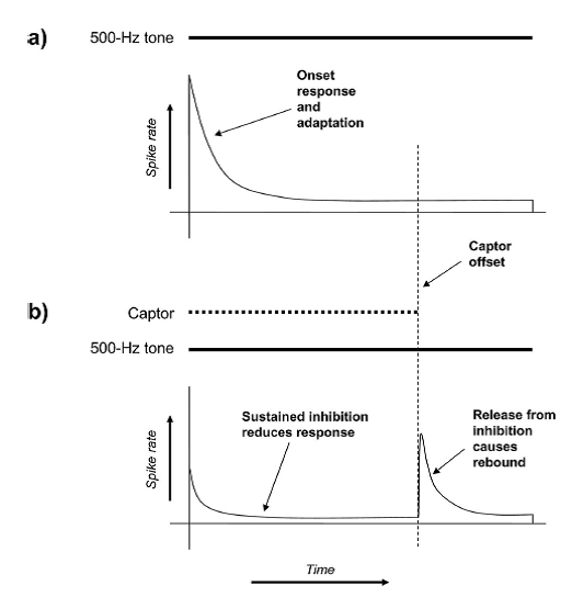
Figure 6.5
Illustration
of the effect of wideband inhibition when a captor tone is used to remove the
effects of onset asynchrony. (A) Responses to the fourth harmonic (at 500 Hz) consist of an onset
burst followed by adaptation to a lower level of activity. (B) In the presence
of the captor, wideband inhibition would reduce the responses to the 500-Hz
tone. Furthermore, at the offset of the captor tone, neurons receiving wideband
inhibition tend to respond with a rebound burst (as shown by Bleeck et al. 2008).
From figure
2 in Holmes and Roberts (2006).
Wideband inhibition could supply
an alternative low-level account of the effects of the captor tone (figure
6.5). When the captor tone is played, it could (together
with the 500-Hz tone) activate wideband inhibition, which in turn would reduce
the responses of cochlear nucleus neurons responding to 500 Hz, which would
consequently fire less but therefore also experience less spike rate
adaptation. When the 1,000-Hz captor stops, the wideband inhibition ceases, and
the 500-Hz neurons would generate a “rebound” burst of activity. Because the 1,000-Hz
captor ends when the vowel starts, the rebound burst in the 500-Hz neurons
would be synchronized with the onset bursts of the various neurons that respond
to the harmonics of the vowel, and the fact that these harmonics, including the
500-Hz tone, all fired a burst together will make it look as if they had a
common onset.
Thus, once again we see that it
may be possible to account for a high-level “cognitive” phenomenon in terms of
relatively low-level mechanisms. Support for such low-level accounts comes from
recent experiments by Holmes and Roberts (2006; Roberts & Holmes, 2006,
2007). For example, wideband inhibition is believed to be insensitive to
harmonic relationships, and indeed it turns out that captor tones don’t have to
be harmonically related to the 500-Hz tone. They can even consist of narrow noisebands rather than pure tones. Almost any sound capable
of engaging wideband inhibition will do. The captor tones can even be presented
to the contralateral ear, perhaps because wideband
inhibition can operate binaurally as well as monaurally. Furthermore, there are
physiological results that are consistent with the role of the wideband
inhibitor in this context: Bleeck et al. (2008)
recorded single-neuron responses in the cochlear nucleus of guinea pigs, and
demonstrated the presence of wideband inhibition, as well as the resulting
rebound firing at captor offset, using harmonic complexes that were quite
similar to those used in the human experiments.
But this does not mean that we can
now give a complete account of these auditory grouping experiments in terms of
low-level mechanisms. For example, Darwin and Sutherland (1984) already
demonstrated that increasing the duration of the 500-Hz tone beyond vowel
offset also changes the effect it has on the perceived vowel, and these offset
effects cannot be accounted for either by adaptation or by wideband inhibition.
Thus, there may be things left to do for high-level mechanisms. In this section,
however, it has hopefully become clear that any such high-level mechanisms will
operate on a representation that has changed from the output of the auditory
nerve. For example, adaptation, wideband inhibition, and rebounds will
emphasize onsets and offsets, and suppress responses to steady-state sounds.
Each of the many processing stations of the auditory pathway could potentially
contribute to auditory scene analysis (and, of course, all other auditory
tasks). The information that reaches the high-level mechanisms reflects the
activity in all of the preceding processing stations. For a complete
understanding of auditory scene analysis, we would like to understand what each
of these processing stations does and how they interconnect. This is obviously
an enormous research task.
6.3.2 Fundamental Frequency
and Harmonicity
We will illustrate the
role of pitch and harmonicity in auditory scene
analysis by using a familiar task—separating the voices of two simultaneous
talkers. Here we discuss a highly simplified, yet perceptually very demanding
version of this, namely, the identification of two simultaneously presented
vowels.
In such a double-vowel experiment,
two vowels are selected at random from five or six possible vowels (e.g., /a/,
/e/, /i/, /o/, /u/, or close language-adjusted
versions). The two chosen vowels are then presented simultaneously, and the
subject has to identify both (Sound Example "Double Vowels" on the
book's Web site <flag>). The vowels would be easily discriminated if
presented one after the other, but subjects make a lot of errors when asked to
identify both when they are presented together. With five possible vowels, when
subjects cannot make much headway by simply guessing, their performance would
be only around 4% correct identification for both vowels. When both vowels have
the same pitch, identification levels are in fact substantially above chance (figure
6.6): Depending on the experiment, correct identification
rates may be well above 50%. Still, although well above chance, this level of
performance means that, on average, at least one member of a pair is
misidentified on every other stimulus presentation—identifying double vowels is
a hard task.
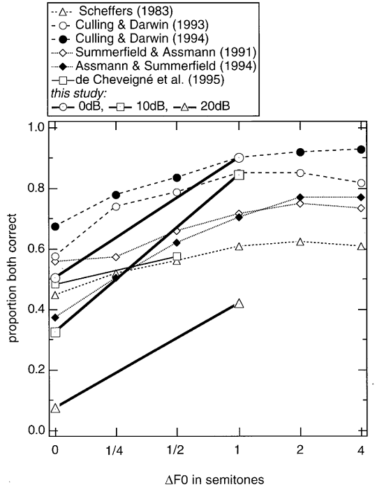
Figure 6.6
Summary
of a number of studies of double vowel identification. The abscissa represents the
difference between the fundamental frequencies of the two vowels. The ordinate
represents the fraction of trials in which both vowels were identified
correctly. The data from de Cheveigné et al. (1997a)
represents experiments in which the two vowels had different sound levels (as
indicated in the legend). The difference in fundamental frequency was as
useful, or even more useful, for the identification of vowels with different
sound levels, a result that is inconsistent with pure-channel selection and may
require harmonic cancellation, as discussed in the main text.
From figure 1 of de Cheveigné et al. (1997).
The main manipulation we are
interested in here is the introduction of a difference in the fundamental
frequency (F0) of the two
vowels. When the two vowels have different F0s,
correct identification rates increase (figure 6.6),
at least for F0
differences of up to 1/2 semitone (about 3%). For larger differences in F0, performance saturates.
Thus, vowels with different F0s
are easier to discriminate than vowels with the same F0.
What accounts for this improved
performance? There are numerous ways in which pitch differences can help vowel
segregation. For example, since the energy of each vowel is not distributed
equally across frequency, we would expect the responses of some auditory nerve
fibers to be dominated by one vowel and those of other fibers to be dominated by
the other vowel. But since the activity of auditory nerve fibers in response to
a periodic sound is periodic (see chapter 3), those fibers whose activity is
dominated by one vowel should all fire with a common underlying rhythm, because
they all phase lock to the fundamental frequency of that vowel. If the vowels
differ in F0, then each
vowel will impose a different underlying rhythm on the population of nerve
fibers it activates most strongly. Thus, checking the periodicity of the
responses of each auditory nerve fiber should make it possible to assign
different fibers to different vowels, and in this way to separate out the
superimposed vowel spectra. Each vowel will dominate the activity of those
fibers whose best frequency is close to the vowel’s formant frequencies. Thus,
the best frequencies of all the fibers that phase lock to the same underlying periodicity
should correspond to the formant frequencies of the vowel with the
corresponding F0. This
scheme is called “channel selection”.
The plausibility of channel
selection has indeed been demonstrated with neural activity in the cochlear
nucleus (Keilson et al. 1997). This study looked at
responses of “chopper” neurons in the cochlear nucleus to vowel sounds. Chopper
neurons are known to phase lock well to the F0
of a vowel. In this study, two different vowels were used, one /I/, and one /ae/, and these were embedded within the syllables /bIs/ or /baes/. The /I/ had a F0 of 88 Hz, the /ae/ a slightly higher F0
of 112 Hz. During the experiment, the formants of the /I/ or the /ae/ sounds were tweaked to bring them close to the best
frequency (BF) of the recorded chopper neuron. Figure 6.7A
shows the response of the neuron to the /I/ whose second formant frequency was
just above the neuron’s BF. The left column shows the instantaneous firing rate
of the neuron during the presentation of the syllable. The horizontal line
above the firing rate histogram shows when the vowel occurred. Throughout the
stimulus, the neuron appears to fire with regular bursts of action potentials,
as can be seen from the peaks in the firing rate histogram. The right column
shows the frequency decomposition of the firing rate during the vowel
presentation. The sequence of peaks at 88 Hz and its multiples demonstrate that
the neuron indeed emitted a burst of action potentials once every period of the
vowel. Figure 6.7D
(the bottom row), in comparison, shows the responses of the same neuron to the
/ae/ sound with the slightly higher F0. Again, we see the neuron
responds with regular bursts of action potentials, which are synchronized this
time to the stimulus F0 of
112 Hz (right dot).
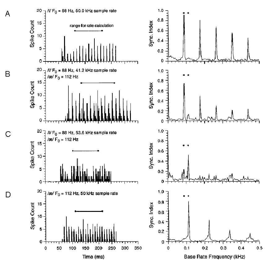
Figure 6.7
(A and D) Responses of a chopper neuron to the syllables /bIs/
and /baes/ with F0
or 88 or 112 Hz, respectively. (B and C) Responses of the same neuron to
mixtures of /bIs/ and /baes/
presented at the same time. The plots on the left show poststimulus
time histograms (PSTHs) of neural discharges,
representing the instantaneous firing rate of the neuron during stimulus
presentation. The lines above the PSTHs indicate when
the vowels /I/ and /ae/ occurred during the
syllables. The plots on the right are the frequency decompositions of the PSTHs during vowel presentation, measuring the locking to
the fundamental frequency of the two vowels: A sequence of peaks at 88 Hz and
its multiples indicate locking to the fundamental frequency of the /I/ sound,
while a sequence of peaks at 112 Hz and its multiples indicate locking to the
fundamental frequency of the /ae/ sound. The two
fundamental frequencies are indicated by the dots above each panel.
From figure
3 of Keilson et al. (1997).
The two middle rows, figures
6.7B and C, show
responses of the same neuron to “double vowels,” that is, different mixtures of
/I/ and /ae/. The firing patterns evoked by the mixed
stimuli are more complex; However, the plots on the right clearly show that the
neuron phase locks either to the F0
of the /I/ of 88 Hz (figure 6.7B) or to
the F0 of the /ae/ of 112 Hz (figure
The temporal discharge patterns
required to make channel selection work are clearly well developed in the
cochlear nucleus. But is this the only way of using periodicity? A substantial
amount of research has been done on this question, which cannot be fully
reviewed here. We will discuss only a single thread of this work—the somewhat
unintuitive idea that pitch is used to improve discrimination is by allowing
harmonic cancellation (de Cheveigné,
1997; de Cheveigné et al., 1995, 1997a, 1997b).
Effectively, the idea is that the periodicity of one vowel could be used to
remove it from a signal mixture, and the remainder could then be examined to
identify further vowels or other background sounds. One very simple circuit
that implements such a scheme is shown in figure 6.8A.
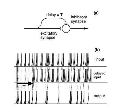
Figure 6.8
A
cancellation filter. (A) The neural architecture. The same input is fed to the neuron
through an excitatory synapse and through an inhibitory synapse, with a delay, T, between them. As a result, any spike
that appears exactly T seconds
following another spike is deleted from the output spike train. (B) An example
of the operation of the cancellation filter. Only
spikes that are not preceded by another spike T seconds earlier appear in the output.
From figure
1 of de Cheveigné (1997a).
The inhibitory
delay line shown in figure 6.8A acts as a filter that deletes
every spike that occurs at a delay T
following another spike. If the filter is excited by a periodic spike train with a period T, the output rate would be
substantially reduced. If the spike train contains two superimposed trains of
spikes, one with a period of T and
the other with a different period, the filter would remove most of the spikes
that belong to the first train, while leaving most of the spikes belonging to
the other. Suppose now that two vowels are simultaneously presented to a
subject. At the output of the auditory nerve, we position two cancellation
filters, one at a delay corresponding to the period of one vowel, the other at
the period of the other vowel. Finally, the output of each filter is simply
quantified by its rate—the rate of the leftover spikes, after
canceling those that presumably were evoked by the other vowel.
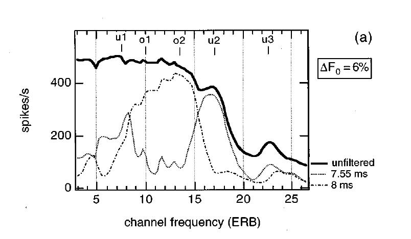
Figure 6.9
A simulation of
cancellation filters. The thick black line represents the overall firing rate
of auditory nerve fibers stimulated by a double vowel consisting of /o/ and /u/
played simultaneously. The thin lines represent the output of cancellation
filters, one at the pitch of each of the two vowels, positioned at the output
of each auditory nerve fiber. The representation of the formants is recovered
at the output of the cancellation filters.
From figure
3a of Cheveigné et al. (1997a).
The results of
such a process is illustrated in figure 6.9,
which is derived from a simulation. The two vowels in this example are /o/ and
/u/. The vowel /o/ has a rather high first formant and a rather low second
formant (marked by o1 and o2 in figure 6.9),
while /u/ has a lower first formant and a higher second formant (marked by u1
and u2). The thick line represents the rate of firing of the auditory nerve
fiber array in response to the mixture of /o/ and /u/. Clearly, neither the
formants of /o/ nor those of /u/ are clearly represented. The dashed lines are
the rates at the output of two cancellation filters, tuned to the period of
each of the two vowels. The vowel /u/ had an F0 of 125 Hz, with a period of 8 ms; /o/ had an F0 of 132 Hz, with a period
of about 7.55 ms. Thus, the cancellation filter with a period of 8 ms is
expected to cancel the contribution of /u/ to the firing rate, and indeed the
leftover rate shows a broad peak where the two formants of /o/ lie. Conversely,
the cancellation filter with a period of 7.55 ms is expected to cancel the
contribution of /o/ to the firing rate, and indeed the leftover rate has two
peaks at the locations of the formant frequencies of /u/. So the cancellation
scheme may actually work.
Now we have two mechanisms that
may contribute to double-vowel identification: channel selection and
periodicity cancellation. Do we need both? De Cheveigné
and his colleagues investigated the need for periodicity cancellation in a
number of experiments. One of them consisted of testing the discriminability,
not just of periodic vowels, but also of nonperiodic
vowels (de Cheveigné et al., 1995; De Cheveigné et al., 1997b). The latter were produced by
shifting their harmonics a bit. This creates an aperiodic
sound that has a poorly defined pitch, but nevertheless a clear vowel identity
(Sound Example "Inharmonic Vowels" on the book's Web site
<flag>). When periodic and aperiodic vowels are
presented together, only the periodic vowels can be canceled with the scheme
proposed in figure 6.8, but the aperiodic vowel should nevertheless be clearly represented
in the “remainder.” Indeed, aperiodic vowels could be
more easily discriminated in double-vowel experiments with mixtures of periodic
and aperiodic vowels. That result can be easily
explained with the cancellation idea, but is harder to explain in terms of
channel selection. The channels dominated by the aperiodic
vowels would presumably lack the “tagging” by periodicity, and therefore
nothing would link these channels together. Thus, channel selection alone
cannot explain how inharmonic vowels can be extracted from a mixture of sounds.
Another line of evidence that
supports the cancellation theory comes from experiments that introduce sound
intensity differences between the vowels. A rather quiet vowel should
eventually fail to dominate any channel, and the channel selection model would
therefore predict that differences of F0
would be less useful for the weaker vowel in a pair. Harmonic cancellation
predicts almost the opposite: It is easier to estimate the F0 of the higher-level vowel and hence to cancel it in
the presence of F0
differences. Consequently, the identification of the weak vowel should benefit
more from the introduction of F0
differences. Indeed, de Cheveigné and colleagues
(1997a) demonstrated that the introduction of differences in F0 produced a greater benefit
for identifying the weaker than the louder vowel in a pair (see figure
6.6 for some data from that experiment). Thus, the overall
pattern of double-vowel experiments seems to support the use of harmonic
cancellation.
But is there any physiological
evidence for harmonic cancellation operating in any station of the auditory
pathway? In the cochlear nucleus, we have seen that chopper neurons tend to be
dominated by the periodicity of the vowel that acoustically dominates their
input. Other kinds of neurons seem to code the physical complexity of the
mixture stimulus better, in that their responses carry evidence for the
periodicity of both vowels. However, there is no evidence for cochlear nucleus
neurons that would respond preferentially to the weaker vowel in a pair, as might be expected from cancellation. The
same is true in the inferior colliculus (IC), as was
shown by Sinex and colleagues (Sinex
& Li, 2007). Neurons in the central nucleus of the IC are sensitive to the
composition of the sound within a narrow frequency band around their best
frequency; when this band contains harmonics of both vowels, their activity
would reflect both periodicities. Although IC neurons have not been tested with
the same double-vowel stimuli used by Keilson et al.
(1997) in the cochlear nucleus (figure
6.7), the available data nevertheless indicates that
responses of the neurons in inferior colliculus would
follow pretty much the same rules as those followed by cochlear nucleus
neurons. Thus, we would not expect IC neurons to show cancellation of one vowel
or the other. Other stations of the auditory pathways have not been tested with
similar stimuli. Admittedly, none of these experiments is a critical test of
the cancellation filter. For example, cancellation neurons should have “notch”
responses to periodicity—they should respond to sounds of all periodicities
except around the period they preferentially cancel. None of the above
experiments really tested this prediction.
What are we to make of all this?
Clearly, two simultaneous sounds with different F0s are easier to separate than two sounds with the same
F0. Thus, periodicity is
an important participant in auditory scene analysis. Furthermore,
electrophysiological data from the auditory nerve, cochlear nucleus, and the IC
indicate that, at least at the level of these stations, it may be possible to
improve vowel identification through channel selection by using the periodicity
of neural responses as a tag for the corresponding channels. On the other hand,
psychoacoustic results available to date seem to require the notion of harmonic
cancellation—once you know the periodicity of one sound, you “peel” it away and
study what’s left. However, there is still no good electrophysiological
evidence for harmonic cancellation.
To a large degree, therefore, our
electrophysiological understanding lags behind the psychophysical results. The
responses we see encode the physical structure of the double-vowel stimulus,
rather than the individual vowels; they do so in ways that may help disentangle
the two vowels, but we don’t know where and how that process ends.
Finally, none of these models
offers any insight into how the spectral profiles of the two vowels are
interpreted and recognized (de Cheveigné & Kawahara,
1999). That stage belongs to the phonetic processing we discussed in chapter 4,
but it is worth noting here that the recovered spectra from double-vowel
experiments would certainly be distorted, and could therefore pose special
challenges to any speech analysis mechanisms.
6.3.3 Common Interaural
Time Differences
Interaural time
differences (ITDs) are a major cue for determining the azimuth of a sound
source, as we had seen in chapter 5. When a sound source contains multiple
frequency components, in principle all of these components share the same ITD,
and therefore common ITD should be a good grouping cue. However, in contrast
with common onsets and harmonicity, which are indeed
strong grouping cues, common ITD appears not to be.
This is perhaps surprising,
particularly since some experiments do seem to indicate a clear role for ITD in
grouping sounds. For example, Darwin and Hukin (1999)
simultaneously presented two sentences to their participants. The first
sentence was an instruction of the type “Could you please write the word bird down now,” and the second was a distractor like “You will also hear the sound dog this time.” The sentences were
arranged such that the words “bird” and “dog” occurred at the same time and had
the same duration (Sound Example "ITD in the Perception of Speech" on
the book's Web site <flag>). This created confusion as to which word (bird
or dog) was the target, and which the distractor. The
confusion was measured by asking listeners which word occurred in the target
sentence (by pressing b for “bird” or
d for “dog” on a computer keyboard),
and scoring how often they got it wrong. Darwin and Hukin
then used two cues, F0 and
ITD, to reduce this confusion. They found that, while rather large F0 differences reduced the
confusion by only a small (although significant) amount, even small ITDs (45 μs left ear–leading for one sentence, 45 μs right ear–leading for the other one) reduced the
confusion by substantially larger amounts. Furthermore, Darwin and Hukin pitted F0
and ITD against each other, by presenting the sentences, except for the target
word “dog,” with different F0s,
and making the F0 of the
target word the same as that of the distractor
sentence. They then played these sentences with varying ITDs, and found that
ITD was actually more powerful than F0
– in spite of the difference in F0
between the target word and the rest of the sentence, listeners were
substantially more likely to associate the word with the rest of the sentence,
presumably because both had the same ITD. This experiment suggests that ITD has
a powerful role in linking sequential sounds—we tend to associate together
elements of sounds that occur sequentially with the same ITD. However, this is
a different situation from the one we have been discussing so far, where we
studied cues for grouping acoustic components that overlap in time. So what is
the role of ITD in simultaneous
grouping?
The fact that ITD is only a weak
cue for simultaneous grouping was reported initially by Culling and Summerfield
(1995). We will describe here a related experiment that shows the same type of
effects, using a phenomenon we described earlier when discussing the role of
common onsets: the shifts in the category boundary between /I/ and /e/ due to
the manipulation of one harmonic. We have already discussed the role of onset
asynchrony in modifying the degree of fusion of a harmonic with the rest of the
tone complex. Let us now consider a similar experiment by Darwin and Hukin (1999), which shows that ITDs exercise a much smaller
influence on the perceptual fusion of frequency components than common onsets.
As in the study of onset
asynchrony, Darwin and Hukin (1999) generated a set
of vowels spanning the range between /I/ and /e/ by modifying the first
formant. The vowels had a constant pitch of 150 Hz. Then, they extracted the
600-Hz (fourth) harmonic of the vowel, and presented the vowel without its fourth
harmonic at one ITD, and the missing harmonic separately with either the same
or a different ITD. Perhaps surprisingly, changing the ITD of this harmonic had
no effect on whether the vowel was perceived as an /I/
and /e/, even though we might have expected that changing the ITD of the fourth
harmonic would separate it from the rest of the vowel, and thereby change its formants.
To further demonstrate the lack of effect of ITD on simultaneous grouping,
Darwin and Hukin repeated a manipulation we already
met—increasing the level of the fourth harmonic, which made more of the vowels
sound like /e/, since this manipulation shifted the first formant peak to
higher values. As before, they tried now to reduce the effect of the higher
level of the fourth harmonic by changing its ITD (similarly to the attempt to
reduce the effect of harmonic level by manipulating its onset). But the effects
of increasing the level of the fourth harmonic were essentially the same,
regardless of whether or not it had the same ITD as the rest of the vowel. ITD
therefore seems not to operate as a simultaneous grouping cue, or at least it
cannot ungroup simultaneous frequency components that have been grouped on the
basis of common onset and harmonicity.
How do we understand the seemingly
contradictory results of the two experiments? Darwin and Hukin
suggested that the role of the sentence in the dog versus bird experiment was
to direct the auditory system to process auditory objects from a specific
location in space, leading to the strong effect of ITD, not because of its
intrinsic properties, but because it suggested that the word occurred in the
same spatial location. In the second experiment, there was no such cuing, and
therefore other acoustic cues (e.g., harmonicity)
overrode the effects of ITD.
6.3.4 Neural Correlates
of Simultaneous Segregation and Grouping
Although this section has
presented a number of neural correlates of segregation of simultaneous sounds
and possible mechanisms that contribute to this goal, we did not mention many
neural correlates of the actual endpoint of this process—the representation of
the segregated sounds. The reason for this is simple: There are very few
examples of this in the literature. One possible example is the case of CMR in
auditory cortex, as described in the previous section. However, CMR is a
somewhat artificial construct. We would really like to be able to show examples
of mixtures of natural sounds being segregated and represented separately
somewhere in the brain.
Some evidence that this may occur
at the level of primary auditory cortex has been offered by Bar-Yosef and colleagues (Bar-Yosef
& Nelken, 2007; Bar-Yosef,
Rotman, & Nelken, 2002;
Nelken & Bar-Yosef,
2008). They studied responses to bird songs extracted from natural recordings.
Because these recordings were made “in the real world,” the songs were
accompanied by additional acoustic components such as echoes and background
noises. It is possible, however, to separate out the “foreground” bird song
from the background noise, and to present separately the cleaned “foreground
only” song or the much quieter remaining background sounds to neurons (Sound
Example "Bird Songs and their Backgrounds" on the book's Web site <flag>).
Figure 6.10 displays the responses of four cat
auditory cortex neurons to these stimuli. The top panel shows the responses of
these neurons to pure tones with different frequencies and levels. These
“frequency response area” (FRA) plots reveal a typical V-shaped tuning curve
with best frequencies around 4 kHz, close to the center frequency of the bird
chirps that were used in these experiments. On top of the FRAs,
the thick dark gray line represents the frequency content of the clean bird
chirp. Below the FRAs, the different stimuli and the
resulting responses are shown. The responses are displayed as rasters—there are twenty repeats of each sound and, in each
repeat, a dot represents the time of occurrence of a spike. The stimuli are
shown as spectrograms (described in chapter 1).
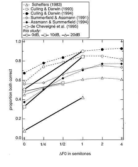
Figure 6.10
Responses
of four neurons to natural bird chirps and their modifications. The top panels display in gray
levels the responses of these neurons to tones of varying frequencies and levels
(along the abscissa and ordinate, respectively), a representation called frequency
response area (FRA). The bottom panels represent the responses of the neurons
to three stimuli: the natural bird chirp (bottom), the clean main chirp (middle),
and the leftover signal (top). In each case, the spectrogram is displayed below
a raster plot, using dots to display the time of occurrence of spikes in twenty
presentations of each of the stimuli. The thick dark gray lines on top of the FRAs represent the frequency content of the clean chirp ('
From figure
13 of Bar-Yosef and Nelken (2007).
Three stimuli are shown for each
neuron. The bottom stimulus is a segment from a natural recording, including
the bird chirp and all the rest of the sound, which includes echoes (the ”halo” around the chirps) and rustling (apparent as a
mostly uniform background at all frequencies). The middle stimulus is the
“foreground only” bird chirp, and the upper stimulus is the remainder after
removal of the chirp, that is, just the echoes and background. Considering that
most of the sound energy of the original, natural sound is contained in the
bird chirp, the responses to the original recording and the cleaned chirp
(bottom and middle rows) can be surprisingly different. In fact, in the
examples shown here, the responses to the background, played alone, were much
more similar to the responses to the full natural stimulus than were the
responses to the foreground only stimulus.
The responses of these neurons may
be interpreted as correlates of the end point of a process of scene
analysis—they respond to some, but not all, of the components of an auditory
scene. In fact, they respond to the weaker components in the scene. Perhaps
other neurons respond to the clean chirp rather than to the background,
although Bar-Yosef and Nelken
(2007) did not describe such neurons. Alternatively, it may be that these
neurons are really doing the hard part of auditory scene analysis—the
foreground bird chirp is easy to hear. Hearing the background is harder, but
potentially very important: The sounds of prey or predators may lie hidden in
the background! Surveillance of the subtler background sounds might be a key
function of auditory cortex. In fact, the same group presented data suggesting
that responses in IC to these sounds are usually more closely related to the
physical structure of the sounds, and therefore more strongly influenced by the
high-intensity foreground. Thalamic responses, on the other hand, would appear
to be more similar to the cortical responses (Chechik
et al., 2006). So far, however, there are only very few such examples in the
literature. Much more experimental data with additional stimuli will be
required to fully assess the role of cortex in auditory scene analysis.
6.4 Nonsimultaneous Grouping and Segregation: Streaming
Simultaneous grouping
and segregation is only one part of auditory scene analysis. Sound sources are
often active for a long time, and the way they change (or not) as a function of
time has important consequences for the way they are perceived. We already
encountered an effect of this kind—the effect of ITD on grouping, which was
large for sequential sounds but weak for simultaneous grouping.
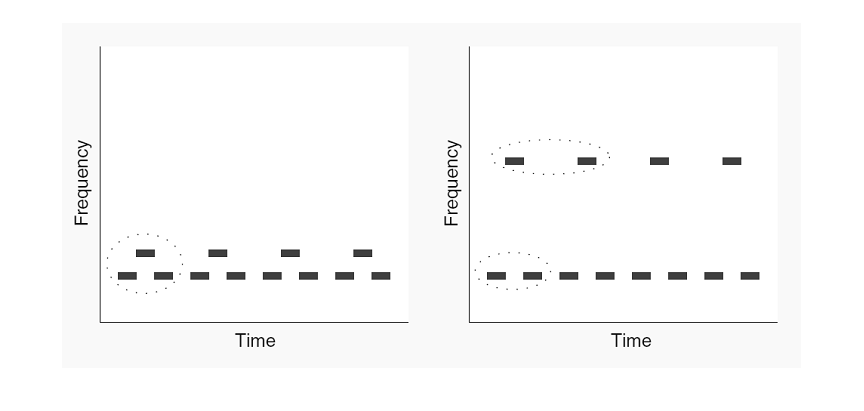
Figure 6.11
Streaming is the
breakdown of a sequence of tones into two “streams.” In this illustration,
tones of two frequencies are presented successively, with the higher tone at
half the rate of the lower one. When the frequency separation between the two
is small, the result is a single stream of sounds with a basic three-tone
galloping melody. When the frequency separation between the two tones is large,
the sequence breaks down into two streams, one composed of the low-frequency
tones, the other of the high-frequency tones.
From figure
1 of Schnupp (2008)[DH1] .
A number of examples of this kind
have been studied in the literature. Possibly the simplest form of streaming
uses two pure tones (Sound Example "Streaming with Alternating Tones"
on the book's Web site <flag>). The two tones are played alternately at a
fixed rate. If the rate of presentation is slow and the interval between the
two tones is small, the result is a simple melody consisting of two alternating
tones. However, if the rate of presentation is fast enough and the frequency
separation between the two tones is large enough, the melody breaks down into
two streams, each consisting of tones of one frequency. A more interesting
version of the same phenomenon, which has been studied intensively recently, is
the “galloping,” or “
The breakdown of a sequence of
sounds into two (or possibly more) things is called “streaming,” and we can
talk about perception of one (at slower presentation rates) or two (at faster
presentation rates) streams. Later, we will discuss the relationships between
these things and auditory objects, which we introduced earlier in the chapter.
The study of streaming was popularized by Al Bregman
in the 1970s, and is described in great detail in his highly influential book Auditory Scene Analysis (Bregman, 1990). Importantly, the attempts
of Bregman to justify the claim that there are
multiple perceptual things, which he called streams, are described in that book
and will not be repeated here.
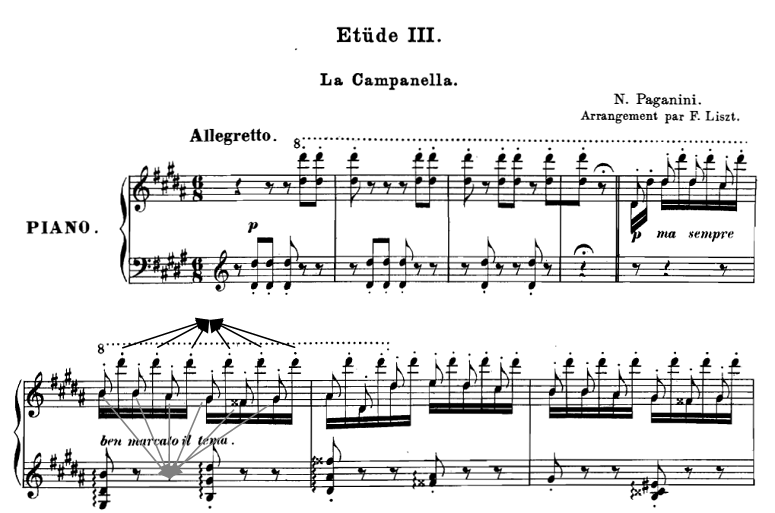
Figure 6.12
The
beginning of La Campanella etude from Liszt’s “Large
Paganini Studies.” The melodic line consists of the low tones in the pianist’s right
hand, which alternates with high tones, up to two octaves above the melodic
line. The melody streams out in spite of the alternations with the high tones.
The gray and black arrows indicate the notes participating in the two streams
in one bar.
Streaming in this form has been
used in classical music to create multiple musical lines with instruments that
can produce only a single pitch at a time. The best known examples are probably
from the Baroque period—for example, J. S. Bach in his compositions for solo
violin famously used such melodies, composed of alternating high and low tones.
These melodies split apart into two separate, simultaneous melodic lines, thus
enriching the musical texture. Another rather well-known example is from
Liszt’s La Campanella etude, which is a free
adaptation of the main theme of the last movement of Paganini’s second violin
concerto (figure 6.12 and Sound Example "La
Campanella" on the book's Web site <flag>).
We have already mentioned that certain
conditions, such as slow rhythms with long intervals and a small pitch separation
between the notes, favor the perception of a single stream, while the opposite
conditions, namely, fast presentation rates and large pitch intervals (as in
the La Campanella etude), favor the perception of two
separate streams. But what happens in ”intermediate”
regimes? There is a tendency for the single stream to dominate perception for
the first few seconds, following which the single percept may break up into two
streams. Pressnitzer and Hupé
(2006), who carefully measured the duration of this phase, found that for an
interval of 5 semitones (the interval of a fourth, corresponding to a frequency
ratio of about 4/3), and at a presentation rate of about 8 tones/s, the
duration of the initial single-stream percept was on average about 20 s,
corresponding to 160 tone presentations. Eventually, all subjects ended up
hearing two streams. The eventual splitting of the initial single stream into
two is called the “buildup of streaming.”
However, the story doesn’t end
there. When subjects continued to listen to the sequences for even longer, the
perceived organization could switch again into a single stream, and then split
again, alternating between phases of one and two perceived streams. In fact,
this behavior was very much the same as that found in other bistable perceptual
phenomena (Pressnitzer & Hupé,
2006). Thus, the “buildup” of streaming, that is, the initial split, is only
part of what neural models have to account for—it is also necessary to account
for the further switching between the perception of one and two streams (Denham
& Winkler, 2006).
Streaming occurs in nonhuman
animals as well. Thus, MacDougall-Shackleton et al.
(1998) showed streaming in a bird, the European starling, while Izumi (2002)
observed an analog of streaming in Japanese macaques. In Izumi’s experiment,
the monkeys had to recognize short “melodies” that were played alone or with
additional interleaved distracter tones. If the distractor
tones were positioned in a frequency region that did not overlap that of the
melodies, the monkeys were able to recognize correctly the melodies. If the
distracter tones were positioned in a frequency region that did overlap with
that of the melodies, the monkeys failed to recognize the melodies.
The evidence for streaming in
animals is, however, patchy. Human psychophysics is often compared directly
with animal electrophysiological recordings, with the hope that the operation
and organization of human and animal auditory systems are similar enough to
make this comparison valid and informative. While such comparisons must be
handled with care, they can nevertheless be illuminating. For
example, a basic model for the mechanisms behind streaming was suggested by
Fishman et al. (2001), based on recordings from the auditory cortex of
macaques. The macaques listened passively to a sequence of two
alternating tones (as in Sound Example "Streaming
with Alternating Tones"
<flag>), one of which matched the BF of the neurons under study. An example
of the recorded neuronal responses is illustrated in figure
6.13, which shows the responses of two multiunit clusters
to such sequences. The large, transient increases in firing rates (visible as
peaks in the firing rate histograms) are the responses to the tones. The
presentations of BF tones are marked by open dots and those of the non-BF tones
by filled dots at the bottom of the panels (and by open arrows in the panels
showing the responses to faster sequences). The crucial observation is that, as
sequence rate is increased, the responses to the non-BF tones decrease faster
than the responses to the BF tones. Thus, for example, at a presentation rate
of 20 Hz, the BF tones evoke large responses in both of the recording sites
shown, but the non-BF tone does not evoke any responses in one of them (the
upper panel) and a substantially reduced response in the other (lower panel).
Fishman et al. (2001) suggested that the differential effect of presentation
rate on BF and non-BF tones is the result of “forward masking”—the reduction in
response to a tone due to the presentation of another tone just before.
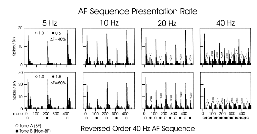
Figure 6.13
A
possible neuronal correlate of streaming. The responses of two neurons to sequences of
alternating tones presented at different rates. One of the two tones was always
at BF, the other at an interval of 40% (top) or 50% (bottom) away. At the
slower presentation rates, both tones evoked responses (e.g., the 5-Hz panels).
However, at faster presentation rates, while the responses to both tones
decreased, the responses to the non-BF tones decreased to a larger degree than those
of the BF tone.
From figure
8 of Fishman et al. (2001).
How do these findings relate to
streaming? Fishman et al. (2001) proposed the following hypothesis: As long as
the majority of responsive neurons are activated by either of the two tones, a
single stream is perceived. In contrast, if one tone evokes a response mostly
in one neuronal population, while the other tone evokes a response mostly in a
different, nonoverlapping neuronal population, two
streams are perceived. Thus, when the frequency separation between the two
tones is large enough, two streams are always perceived. Similarly, if the
frequency separation between the two tones is very small, a single stream is
always observed.
When the frequency separation
between the two tones is intermediate, the rate of presentation becomes an
important factor—slow presentations favor a single stream, because at low
presentation rates there is less forward masking that would suppress responses
to the non-BF tone. Increasing the presentation rate leads to more forward
masking; in consequence, cortical neurons increasingly respond to only one tone
or the other, but not to both. The neuronal populations responding to both
tones tend to overlap less, which in turn favors the perception of the two
tones in separate streams. The data of Fishman et al. (2001) are indeed
compatible with this hypothesis.
This model is appealing, but it
needs to be made quantitative. For example, one would like to know how much the
two populations should overlap in order for a single stream to be perceived. Micheyl et al. (2005) used a nice twist to make this model
quantitative. They decided to study the buildup of streaming—the time it takes
for the initial galloping rhythm to split into two streams. First, they used
At this point, the decline in the
response to the B tone mimics qualitatively the buildup of streaming, but Micheyl et al. (2005) went a step further. Remember that in
this experiment, neurons always respond to the A tone, as that tone is at their
BF. Micheyl and colleagues wanted to have a threshold
such that if the neurons respond to the B tone above this threshold, they would
also participate in the representation of the B tone and, according to the
hypothesis of Fishman et al. (2001), there would be only one stream. On the
other hand, when the response to the B tone is below the threshold, these
neurons would not participate in the representation of the B tones, while
other, similar neurons with a BF near the frequency of the B tone would
presumably respond essentially only to the B tone. The A and the B tones would
then be represented in the activity of nonoverlapping
neural populations, which in turn should favor a two-stream percept.
How can we find such a threshold?
Given a guess for the threshold, one can look back at the data and see how many
times the responses to the B tone are smaller than that threshold—this would be
an estimate for the probability of perceiving one streams rather than two. The
question is, is it possible to find a single threshold
that makes the predicted likelihoods of perceiving one stream, as derived from
the neural recordings, line up with the actual likelihoods measured
experimentally? The curves shown in figure 6.14B
suggest that it is indeed possible to find such a threshold.
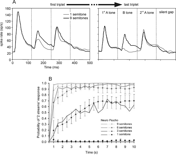
Figure 6.14
(A) Average responses
of ninety-one neurons in the macaque auditory cortex to the
From
figures 2 and 4 of Micheyl et al. (2005).
These studies show that the
dynamic response properties of cortical neurons may account for streaming, but
they fall someway short of a conclusive and complete account of this
phenomenon. A number of critiques and open questions are still to be answered.
One critique states that, while this model accounts for the buildup, it doesn’t
account for the bistability—the switching back and forth between one- and
two-stream percepts. Unfortunately, no physiological study as yet even attempts
to account for the bistability of streaming. A second critique is that, though this
model may be correct, it doesn’t necessarily have to be based on cortical
responses. In fact, neurons as early as the cochlear nucleus show a similar,
although substantially smaller, differential adaptation effect. The effect is
smaller, but the variability in the responses in the cochlear nucleus is also
much smaller, and therefore the same statistical technique used to produce the
fit between monkey cortical responses and human behavior can produce a similar
fit between the responses of neurons in the cochlear nucleus of the guinea pig
and human behavior (Pressnitzer et al., 2008). As we
have seen so often in this chapter, high-level and low-level mechanisms compete
for explaining the same perceptual phenomena.
A third critique is that the
Fishman model has been studied only for streaming based on frequency
differences. However, streaming can be induced by many acoustic differences—for
example, by amplitude modulation rate, which is only very weakly related to
spectral differences (Sound Example "Streaming by Amplitude Modulation
Rate" on the book's Web site <flag>). Whether the same type of
increased differentiation between populations would occur for other acoustic
differences is an open question. Some initial work in this direction shows a
possibility to generalize the Fishman model to amplitude modulation (Itatani & Klump, 2009).
With the recent intensive research
into streaming, the “playground” for relating it to neural responses is now well
delimited. To hazard a guess, the main weakness of all models today is their
inability to account for bistability. Thus, many puzzles remain for future
work, and possibly for new conceptual models as well.
6.5 Nonsimultaneous Grouping and Segregation: Change Detection
You sit in a room
preparing for an exam that is going to take place tomorrow. Music is playing in
the background. Through the windows, sounds from the busy street are heard.
Your roommate is walking in the next room, stepping from one end of the room to
the other, but you ignore all of these sounds, concentrating on your revision.
Then one of your friend’s steps is different—and you are suddenly aware of it.
As we discussed in the first
chapter, sounds provide information about numerous aspects of the world, and
minute changes in sounds, such as the sound of a step on a different material
than we expected, may be highly informative. We are very sensitive to such
changes in the auditory scene. This sensitivity is often studied with a tool
called Mismatch Negativity (MMN). MMN is a component of the so-called auditory
event-related potentials (ERPs), the set of
electrical waves that are evoked by sounds and measured by electroencephalography
(EEG).
MMN is evoked by unexpected sounds
embedded in a stream of expected sounds. It is preattentive:
evoked even without attention. In the simplest version of an experiment for
measuring MMN, the subject is distracted (e.g., by reading a book or watching a
silent movie) while sounds are played by earphones and the EEG is measured. The
sound sequence usually consists of two pure tones that vary in some property: They
may have different frequencies, or different sound levels, or different durations.
One of the two tones is played with high probability (this tone is often called
the standard), while the other is rare (the deviant). The deviant tone is
presented randomly in the sequence, for example, with a probability of 10%.
Under these circumstances, the ERP is somewhat different in response to the
standard and to the deviant: When measuring the potential between the top of
the head and the bottom of the mastoids, the response to the deviant is more
negative than the response to the standard in a time window around 100 to 150
ms after stimulus onset (figure 6.15).
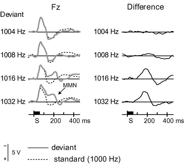
Figure 6.15
Mismatch negativity
(MMN) to frequency deviants. (Left) The potential between
electrode Fz (an electrode on the midline, relatively
frontal) and the mastoid in response to a 1,000-Hz tone (dashed line) that serves
as the standard, and deviant tones at the indicated frequencies. (Right)
The difference waveforms (deviant-standard), showing a clear peak around 150 ms
after stimulus onset. Note that negative potentials are plotted upward in this
figure.
From figure
1 of Naatanen et al. (2007).
MMN can be observed even when the
changes in the sounds are quite subtle. It is sensitive to conjunction of
properties or even to deviations from rather complex rules that might govern
the stimulation sequence. In one of the more complex designs that have been
tested, Paavilainen, Arajarvi,
and Takegata (2007) used a sequence that could have
tones of two frequencies, and these tones were either short or long. Each of
the four possible combinations of tone frequency and tone duration (high-long,
high-short, low-long, and low-short) appeared with equal probability. However,
the sequence (Sound Example "A Tone Sequence Following a Complex
Rule" on the book's Web site <flag>) was constructed so that short
tones were almost always followed by low-frequency tones (which could be either
long or short), and long tones were always followed by high-frequency tones
(which also could be either long or short). From time to time, a tone appeared
that violated these rules (a high-frequency tone followed a short tone, or a
low-frequency tone followed a long tone). These deviant tones evoked MMN
(admittedly, a rather small one). Remarkably, in interviews following the
experiment, the listeners reported that they were not aware of the rules
governing the sequence, nor were they able to work out what the rules were when
prompted, and when the rule was explained to them, they had great difficulty
applying it to detect deviants through a conscious effort. Thus, the MMN
stemmed from a presumably preattentive representation
of the regularities in the sound sequence.
But what can these laboratory
experiments tell us about real-world listening? Going back to the situation
described at the beginning of this section, would our friend’s deviant footstep
evoke MMN? Apparently it does. Winkler and coworkers (2003) measured MMN in subjects
who watched a movie (with sound), and were simultaneously presented with simulated
street sounds. On top of this, the sounds of eleven footsteps were heard. The
sounds of the steps varied a bit from one step to the next, as real steps
would. One of the steps simulated walking on a different surface, and this was
inserted either as the second or tenth in the sequence (Sound Example "A
Naturalistic Sound Sequence with a Deviant" on the book's Web site
<flag>). The subjects were engaged in a task that was related to the
movie, and so they had to ignore the other two sound sources. Winkler et al.
(2003) found that MMN was evoked when the deviant step was the tenth but not
when it was the second in the sequence. Thus, MMN was evoked in spite of the natural
variability in the sounds—presumably, when the deviant step was the tenth, a
representation of the regularity of the footsteps had been generated during the
preceding nine steps, so that the deviant step was detected as such. On the
other hand, when the deviant step was in the second position, no representation
of regularity could have been created, and no MMN occurred.
What do we know about the brain
activity underlying MMN? Since MMN was defined and intensively studied in
humans, while more fine-grained studies, such a single-neuron recordings, can
usually be conducted only in nonhuman animals, it is necessary to show that
MMN, or something similar, occurs in animals. And indeed, a number of studies
that measured auditory evoked potentials in rats (Ruusuvirta,
Penttonen, & Korhonen,
1998), cats (Csepe, Karmos,
& Molnar, 1987), and monkeys (Javitt et al.,
1992) reported brain responses that are similar to MMN. These results open the
road to single neuron studies.
The single-neuron analogs of MMN
are based on a phenomenon that has been studied in vision for some time, but
was only recently imported into auditory research—stimulus-specific adaptation
(SSA). We start with two stimuli, both of which evoke responses of similar
strength. Next, we present one of the two stimuli repeatedly, causing a
reduction in the response (adaptation). Finally, we present the other stimulus.
It is possible that the neuron is really tired of responding—in that case, the
response to the other stimulus would be adapted as well. However, in many cases,
the response to the other stimulus is not adapted at all, or only partially
adapted. In that case, we will say that the adaptation to the first stimulus is
stimulus specific, or that we have SSA.
SSA is interesting, precisely
because it is not really adaptation, which is usually defined as a
use-dependent reduction in responses. If adaptation were really a kind of
use-dependent “fatigue,” then the decline in the neuron’s ability to respond
vigorously should affect all stimuli more or less equally. In stimulus-specific
adaptation, the neuron has tired only of the repetitive, adapting stimulus, but
can still fire vigorously to a different, rare stimulus. A better term would
have been “habituation,” which is used in the psychological literature to
indicate a reduction in responses that may be stimulus specific (Dudai, 2002).
It turns out that SSA is strong in
the auditory midbrain and cortex. Ulanovsky et al.
(2003) used oddball sequences of pure tones, similar to those used in MMN
research, and recorded single-unit responses in auditory cortex of cats. To
demonstrate stimulus-specific adaptation, they used two tones that were very
close in frequency—to within 10% or even 4%, which is the behavioral limit of
frequency discrimination in cats. They then played one of the tones as standard
with the other as deviant. As expected, the neurons adapted to the repetitive
standard tone, and the deviant tone evoked relatively larger responses.
However, how do we know that the neuron does not have larger responses to the
deviant tone because of preference for its frequency (it might be closer to the
neuron’s BF than the standard), rather than any adaptive effects? Ulanovsky et al. (2003) controlled for this issue by
repeating the experiment with the roles of the standard and the deviant
reversed. Since both tones served once as standard and once deviant, any
intrinsic preference for one of the tone frequencies could be discounted. Some
of their results are presented in figure 6.16.
The responses to a tone when it was standard (thick light gray line) were most
often smaller than the responses to the same tone when it was deviant (thick dark
gray line). Thus, the neuron was sensitive to the statistical structure of the
sequence, producing larger responses to rare sounds.
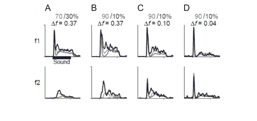
Figure 6.16
Responses
of a neuron in cat auditory cortex to two frequencies (f1 and f2). The frequency difference between
the tones is given at the top of each column, as well as the probabilities of
the two tones. The responses are displayed as peristimulus
time histograms, computed by averaging all the responses to the given frequency
under three conditions: when rare (thick black line), when common (thick gray
line), and when appearing randomly half the time (thin gray line).
From figure
1 in Ulanovsky, Las, and Nelken,
(2003).