5 Neural Basis of Sound Localization
- 5.1 Determining the Direction of a Sound Source
- 5.2 Determining Sound Source Distance
- 5.3 Processing of Spatial Cues in the Brainstem
- 5.4 The Midbrain and Maps of Space
- 5.5 What Does the Auditory Cortex Add?
- 5.6 Localization in More Complex Environments
Most of our senses can
provide information about where things are located in the surrounding
environment. But the auditory system shares with vision and, to some extent,
olfaction the capacity to register the presence of objects and events that can
be found some distance away from the individual. Accurate localization of such
stimuli can be of great importance to survival. For example, the ability to
determine the location of a particular sound source is often used to find
potential mates or prey or to avoid and escape from approaching predators.
Audition is particularly useful for this because it can convey information from
any direction relative to the head, whereas vision operates over a more limited
spatial range. While these applications may seem less relevant for humans than
for many other species, the capacity to localize sounds both accurately and
rapidly can still have clear survival value by indicating, for example, the
presence of an oncoming vehicle when crossing the street. More generally,
auditory localization plays an important role in redirecting attention toward
different sources. Furthermore, the neural processing that underlies spatial
hearing helps us pick out sounds—such as a particular individual’s voice—from a
background of other sounds emanating from different spatial locations, and
therefore aids source detection and identification (more about that in chapter
6). Thus, it is not surprising that some quite sophisticated mechanisms have
evolved to enable many species, including ourselves, to localize sounds with
considerable accuracy.
If you ask someone where a sound
they just heard came from, they are most likely to point in a particular
direction. Of course, pinpointing the location of the sound source also
involves estimating its distance relative to the listener. But because humans,
along with most other species, are much better at judging sound source
direction, we will focus primarily on this dimension of auditory space. A few
species, though, notably echolocating bats, possess specialized neural
mechanisms that make them highly adept at determining target distance, so we
will return to this later.
5.1 Determining the Direction of a Sound Source
Registering the
location of an object that we can see or touch is a relatively straightforward
task. There are two reasons for this. First, the receptor cells in those sensory
systems respond only to stimuli that fall within restricted regions of the
visual field or on the body surface. These regions, which can be extremely
small, are known as the spatial receptive fields of the cells. For example,
each of the mechanoreceptors found within the skin has a receptive field on a
particular part of the body surface, within which it will respond to the
presence of an appropriate mechanical stimulus. Second, the receptive fields of
neighboring receptor cells occupy adjacent locations in visual space or on the
body surface. In the visual system, this is possible because an image of the
world is projected onto the photoreceptors that are distributed around the
retina at the back of the eye, enabling each to sample a slightly different
part of the field of view. As we have seen in earlier chapters, the stimulus
selectivity of the hair cells also changes systematically along the length of
the cochlea. But, in contrast to the receptor cells for vision and touch, the
hair cells are tuned to different sound frequencies rather than to different
spatial locations. Thus, while the cochlea provides the first steps in
identifying what the sound is, it appears to reveal little about where that
sound originated.
Stimulus localization in the
auditory system is possible because of the geometry of the head and external
ears. Key to this is the physical separation of the ears on either side of the
head. For sounds coming from the left or the right, the difference in path
length to each ear results in an interaural difference in the time of sound
arrival, the magnitude of which depends on the distance between the ears as
well as the angle subtended by the source relative to the head (figure
5.1). Depending on their wavelength, incident sounds may
be reflected by the head and torso and diffracted to the ear on the opposite
side, which lies within an “acoustic shadow” cast by the head. They may also
interact with the folds of the external ears in a complex manner that depends
on the direction of sound incidence. Together, these filtering effects produce
monaural localization cues as well as a second binaural cue in the form of a
difference in sound level between the two ears (figure 5.1).
Figure 5.1
Binaural cues for
sound localization. Sounds originating from one side of the head will arrive
first at the ear closer to the source, giving rise to an interaural difference
in time of arrival. In addition, the directional filtering properties of the
external ears and the shadowing effect of the head produce an interaural
difference in sound pressure levels. These cues are illustrated by the waveform
of the sound, which is both delayed and reduced in amplitude at the listener’s
far ear.
Figure 5.2 shows how the different localization
cues vary with sound direction. These measurements were obtained by placing a
very small microphone in each ear canal of a human subject (King, Schnupp,
& Doubell, 2001). The ears are usually pretty symmetrical, so locations
along the midsagittal plane (which bisects the head down the middle, at right
angles to the interaural axis) will generate interaural level differences (ILDs;
figure 5.2A and B)
and interaural time differences (ITDs; figure 5.2C)
that are equal or very close in value to zero. If the sound source shifts from
directly in front (represented by 0° along the horizontal axis of these plots)
to one side, both ILDs and ITDs build up and then decline back toward zero as
the source moves behind the subject. A color version of this figure can be
found in the “spatial hearing” section of the book’s web site <flag>).
ITDs show some variation with
sound frequency, becoming smaller at higher frequencies due to the frequency
dispersion of the diffracted waves. Consequently, the spectral content of the
sound must be known in order to derive its location from the value of the ITD.
However, the ITDs measured for different frequencies vary consistently across
space, with the maximum value occurring on the interaural axis where the
relative distance from the sound source to each ear is at its greatest (figure
5.2C). By contrast, the magnitude of the ILDs changes
considerably with the wavelength and therefore the frequency of the sound.
Low-frequency (long wavelength) sounds propagate around the head with little
interference, and so the resulting ILDs are very small if present at all. This
is illustrated in figure 5.2A for the spatial pattern of
ILDs measured for 700-Hz tone pips; for most locations, the ILDs are around 5
to 10 dB and therefore provide little indication as to the origin of the sound
source. But at higher frequencies, ILDs are larger and, above 3 kHz, become
reliable and informative cues to sound source location. For example, at 11 kHz (figure
5.2B), the ILDs peak at about 40 dB, and show much more
variation with sound source direction. This is partly due to the growing
influence of the direction-dependent filtering of the incoming sound by the
external ears on frequencies above about 6 kHz. This filtering imposes a
complex, direction–dependent pattern of peaks and notches on the sound spectrum
reaching the eardrum (figure 5.2D).
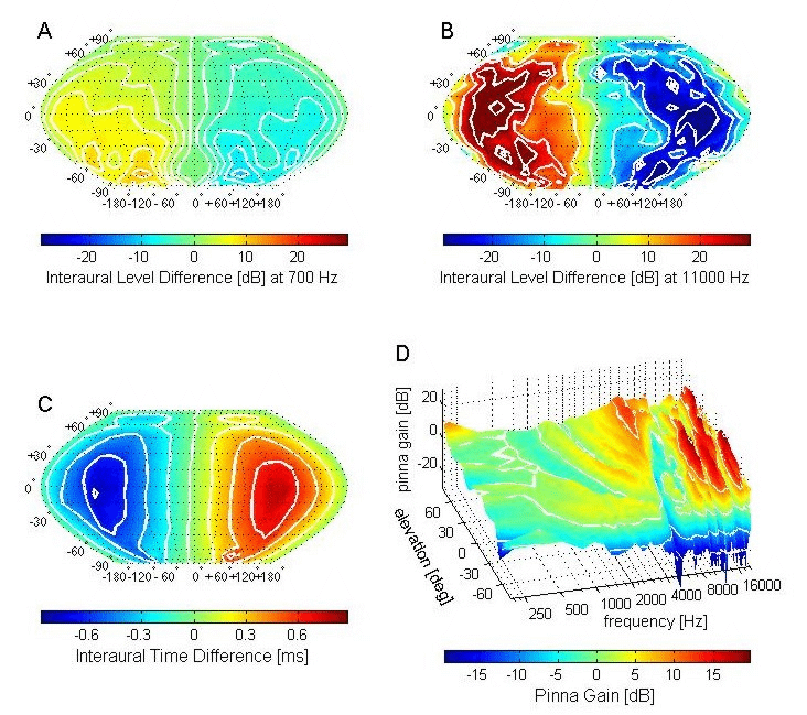
Figure 5.2
Acoustic
cues underlying the localization of sounds in space. (A, B) Interaural level
differences (ILDs) measured as a function of sound source direction in a human
subject for 700-Hz tones (A) and 11-kHz tones (B). (C) Spatial pattern of
interaural time differences (ITDs). In each of these plots, sound source
direction is plotted in spherical coordinates, with 0° indicating a source
straight in front of the subject, while negative numbers represent angles to
the left and below the interaural axis. Regions in space generating the same
ILDs or ITDs are represented by the white lines, which represent iso-ITD and
iso-ILD contours. (D) Monaural spectral cues for sound location. The
direction-dependent filtering effects produced by the external ears, head, and
torso filter are shown by plotting the change in amplitude or gain measured in
the ear canal after broadband sounds are presented in front of the subject at
different elevations. The gain is plotted as a function of sound frequency at
each of these locations.
In adult humans, the maximum ITD
that can be generated is around 700 µs. Animals with smaller heads have access
to a correspondingly smaller range of ITDs and need to possess good
high-frequency hearing to be able to use ILDs at all. This creates a problem
for species that rely on low frequencies, which are less likely to be degraded
by the environment, for communicating with potential mates over long distances.
One solution is to position the ears as far apart as possible, as in crickets,
where they are found on the front legs. Another solution, which is seen in many
insects, amphibians, and reptiles as well as some birds, is to introduce an
internal sound path between the ears, so that pressure and phase differences
are established across each eardrum (figure 5.3).
These ears are known as pressure-gradient or pressure-difference receivers, and
give rise to larger ILDs and ITDs than would be expected from the size of the
head (Christensen-Dalsgaard, 2005; Robert, 2005). For species that use pressure
gradients to localize sound, a small head is a positive advantage as this
minimizes the sound loss between the ears.
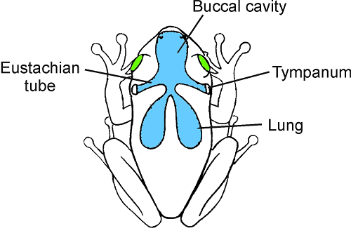
Figure 5.3
In species with pressure-gradient
receiver ears, sound can reach both sides of the eardrum. In frogs, as shown
here, sound is thought to arrive at the internal surface via the eustachian
tubes and mouth cavity and also via an acoustic pathway from the lungs. The
eardrums, which are positioned just behind the eyes flush with the surrounding
skin, are inherently directional, because the pressure (or phase) on either
side depends on the relative lengths of the different sound paths and the
attenuation across the body. This depends, in turn, on the angle of the sound
source.
Mammalian ears are not
pressure-gradient receivers; in contrast to species such as frogs that do use
pressure gradients, mammals have eustachian tubes that are narrow and often closed, preventing sound from
traveling through the head between the two ears. Directional hearing in mammals
therefore relies solely on the spatial cues generated by the way sounds from
the outside interact with the head and external ears. Fortunately, mammals have
evolved the ability to hear much higher frequencies than other vertebrates,
enabling them to detect ILDs and monaural spectral cues, or have relatively large
heads, which provide them with a larger range of ITDs.
Because several physical cues
convey information about the spatial origin of sound sources, does this mean some
of that information is redundant? The answer is no, because the usefulness of each
cue varies with the spectral composition of the sound and the region of space
from which it originates. We have already seen that low frequencies do not
generate large ILDs or spectral cues. In contrast, humans, and indeed most
mammals, use ITDs only for relatively low frequencies. For simple periodic
stimuli, such as pure tones, an interaural difference in sound arrival time is
equivalent to a difference in the phase of the wave at the two ears (figure
5.4), which can be registered in the brain by the
phase-locked responses of auditory nerve fibers. However, these cues are
inherently ambiguous. Note that in figure 5.4,
the ITD corresponds to the distance between the crests of the sound wave
received in the left and right ears, respectively, but it is not a priori
obvious whether the real ITD of the sound source is the time from crest in the
right ear signal to crest in the left (as shown by the little double-headed
black arrow), or whether it is the time from a left ear crest to the nearest
right ear crest (gray arrow). The situation illustrated in figure
5.4 could thus represent either a small, right ear–leading
ITD or a large left ear–leading one. Of course, if the larger of the two
possible ITDs is “implausibly large,” larger than any ITD one would naturally
expect given the subject’s ear separation, then only the smaller of the
possible ITDs need be considered. This “phase ambiguity” inherent in ITDs is therefore
easily resolved if the temporal separation between subsequent crests of the
sound wave is at least twice as long as the time it takes for the sound wave to
reach the far ear, imposing an upper frequency limit on the use of interaural
phase differences for sound localization. In humans, that limit is 1.5 to 1.6
kHz, which is where the period of the sound wave is comparable to the ITD. Consequently,
it may still be difficult to tell whether the sound is located on the left or
the right unless it has a frequency of less than half that value (Blauert,
1997).
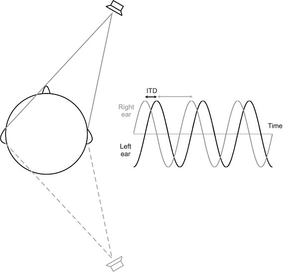
Figure 5.4
The interaural time
delay for a sinusoidal stimulus results in a phase shift between the signals at
each ear. For ongoing pure-tone stimuli, the auditory system does not know at
which ear the sound is leading and which it is lagging. There are therefore two
potential ITDs associated with each interaural phase difference, as shown by
the black and gray arrows. However, the shorter ITD normally dominates our
percept of where the sound. Even so, the same ITD will be generated by a sound
source positioned at an equivalent angle on the other side of the interaural
axis (gray loudspeaker). This cue is therefore spatially ambiguous and cannot
distinguish between sounds located in front of and behind the head.
We can demonstrate the frequency
dependence of the binaural cues by presenting carefully calibrated sounds over
headphones. When identical stimuli are delivered directly to the ears in this
fashion, the sound will be perceived in the middle of the head. If, however, an
ITD or ILD is introduced, the stimulus will still sound as though it originates
inside the head, but will now be “lateralized” toward the ear through which the
earlier or more intense stimulus was presented. If one tone is presented to the
left ear and a second tone with a slightly different frequency is delivered at
the same time to the right ear, the tone with the higher frequency will begin
to lead because it has a shorter period (figure 5.5).
This causes the sound to be heard as if it is moving from the middle of the
head toward that ear. But once the tones are 180° out of phase, the signal
leads in the other ear, and so the sound will shift to that side and then move
back to the center of the head as the phase difference returns to zero. This
oscillation is known as a “binaural beat,” and occurs only for frequencies up
to about 1.6 kHz (Sound Example “Binaural Beats” on the book’s web site
<flag>).

Figure 5.5
Schematic
showing what the interaural phase relationship would be for sound source
directions in the horizontal plane in front of the listener. For source directions to the
left, the sound in the left ear (black trace) leads in time before the sound in
the right ear (gray trace), while for source directions to the right, the right
ear leads. Consequently, tones of slightly different frequencies presented over
headphones to each ear, so that their interaural phase difference constantly shifts
(so-called binaural beat stimuli), may create the sensation of a sound moving
from one side to the other, then “jumping back” to the far side, only to resume
a steady movement. Note that the perceived moving sound images usually sound as
if they move inside the head, between the ears. The rate at which the sound
loops around inside the head is determined by the difference between the two
tone frequencies.
The fact that the binaural cues
available with pure-tone stimuli operate over different frequency ranges was
actually recognized as long ago as the beginning of the twentieth century, when
the Nobel Prize–winning physicist Lord Rayleigh generated binaural beats by
mistuning one of a pair of otherwise identical tuning forks. In an early form
of closed-field presentation, Rayleigh used long tubes to deliver the tones
from each tuning fork separately to the two ears of his subjects. He concluded
that ITDs are used to determine the lateral locations of low-frequency tones,
whereas ILDs provide the primary cue at higher frequencies. This finding has
since become known as the “duplex theory” of sound localization. Studies in
which sounds are presented over headphones have provided considerable support
for the duplex theory. Indeed, the sensitivity of human listeners to ITDs or
ILDs (Mills, 1960; Zwislocki & Feldman, 1956) can account for their ability
to detect a change in the angle of the sound source away from the midline by as
little as 1° (Mills, 1958). This is the region of greatest spatial acuity and,
depending on the frequency of the tone, corresponds to an ITD of just 10 to 15
µs or an ILD of 0.5 to 0.8 dB.
Although listeners can determine
the lateral angle of narrowband stimuli with great accuracy, they struggle to
distinguish between sounds originating in front from those coming from behind
the head (
We must not forget, however, that
natural sounds tend to be rich in their spectral composition and vary in
amplitude over time. (The reasons for this we discussed in chapter 1.) This
means that, when we try to localize natural sounds, we will often be able to
extract and combine both ITD and ILD information independently from a number of
different frequency bands. Moreover, additional cues become available with more
complex sounds. Thus, timing information is not restricted to ongoing phase
differences at low frequencies, but can also be obtained from the envelopes of
high-frequency sounds (Henning, 1974). Broadband sound sources also provide the
auditory system with direction-dependent spectral cues (figure
5.2D), which are used to resolve front-back confusions, as
illustrated by the dramatic increase in these localization errors when the
cavities of the external ears are filled with molds (Oldfield & Parker,
1984).
The spectral cues are critical for
other aspects of sound localization, too. In particular, they allow us to
distinguish whether a sound comes from above or below. It is often thought that
this is a purely monaural ability, but psychophysical studies have shown that
both ears are used to determine the vertical angle of a sound source, with the
relative contribution of each ear varying with its horizontal location (Hofman &
Van Opstal, 2003; Morimoto, 2001). Nevertheless, some individuals who are deaf
in one ear can localize pretty accurately in both azimuth and elevation
(Slattery & Middlebrooks, 1994; Van Wanrooij & Van Opstal, 2004). To
some extent, this can be attributed to judgments based on the variations in
intensity that arise from the shadowing effect of the head, but there is no doubt
that monaural spectral cues are also used under these conditions. The fact that
marked individual variations are seen in the accuracy of monaural localization
points to a role for learning in this process, an issue we shall return to in chapter
7.
Because front-back discrimination
and vertical localization rely on the recognition of specific spectral features
that are imposed by the way the external ears and head filter the incoming
stimulus, the auditory system is faced with the difficulty of dissociating
those features from the spectrum of the sound source itself. Indeed, if
narrowband sounds are played from a fixed loudspeaker position, the perceived
location changes with the center frequency of the sound, indicating that
specific spectral features are associated with different directions in space
(Musicant & Butler, 1984). But even if the sounds to be localized are
broadband, pronounced variations in the source spectrum will prevent the
extraction of monaural spectral cues (Wightman & Kistler, 1997).
Consequently, these cues provide reliable spatial information only if the
source spectrum is relatively flat, familiar to the listener, or can be
compared between the two ears.
It should be clear by now that to pinpoint
the location of a sound source both accurately and consistently, the auditory
system has to rely on a combination of spatial cues. It is possible to measure
their relative contributions to spatial hearing by setting the available cues
to different values. The classic way of doing this is known as time-intensity
trading (Sound Example “Time-Intensity Trading” on the book’s web site
<flag>) (Blauert, 1997). This involves presenting an ITD favoring one ear
together with an ILD in which the more intense stimulus is in the other ear.
The two cues will therefore point to opposite directions. But we usually do not
hear such sounds as coming from two different directions at the same time.
Instead, we typically perceive a sort of compromise sound source direction,
somewhere in the middle. By determining the magnitude of the ILD required to
pull a stimulus back to the middle of the head in the presence of an opposing
ITD, it is possible to assess the relative importance of each cue. Not
surprisingly, this depends on the type of sound presented, with ILDs dominating
when high frequencies are present.
Although presenting sounds over
headphones is essential for measuring the sensitivity of human listeners or
auditory neurons to binaural cues, this approach typically overlooks the
contribution of the spectral cues in sound localization. Indeed, the very fact
that sounds are perceived to originate within the head or at a position very
close to one or the other ear indicates that localization per se is not really
being studied. If the filter properties of the head and external ears—the
so-called head-related transfer function—are measured and then incorporated in
the signals played over headphones, however, the resulting stimuli will be externalized,
that is, they will sound as though they come from outside rather than inside
the head (Hartmann & Wittenberg, 1996; Wightman & Kistler, 1989). The
steps involved in generating virtual acoustic space (VAS) stimuli, which can be
localized just as accurately as real sound sources in the external world (Wightman
& Kistler, 1989), are summarized in figure 5.6 (Sound
Example “Virtual Acoustic Space” on the book’s web site <flag>).
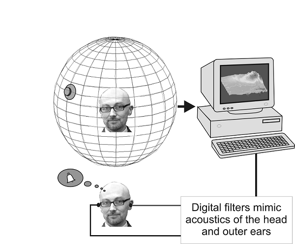
Figure 5.6
Construction
of virtual acoustic space. Probe tube microphones are inserted into the ear canal of the subject,
and used to measure the directional filtering properties of each ear. Digital
filters that replicate the acoustical properties of the external ears are then
constructed. With these digital filters, headphone signals can be produced that
sound as though they were presented out in space.
You might ask why we would want to
go to so much trouble to simulate real sound locations over headphones when we
could just present stimuli from loudspeakers in the free field. This comes down
to a question of stimulus control. For example, one of the great advantages of
VAS techniques is that ITDs, ILDs, and spectral cues can be manipulated largely
independently. Using this approach, Wightman and Kistler (1992) measured
localization accuracy for stimuli in which ITDs signaled one direction and ILDs
and spectral cues signaled another. They found that ITDs dominate the
localization of broadband sounds that contain low-frequency components, which
is in general agreement with the duplex theory mentioned previously. Nevertheless,
you may be aware that many manufacturers of audio equipment have begun to
produce “surround-sound” systems, which typically consist of an array of perhaps
five mid- to high-frequency loudspeakers, but only a single “subwoofer” to
deliver the low frequencies. These surround-sound systems can achieve fairly
convincing spatialized sound if the high-frequency speaker array is correctly
set up. But since there is only one subwoofer (the positioning of which is
fairly unimportant), these systems cannot provide the range of low-frequency
ITDs corresponding to the ILDs and spectral cues available from the array of
high-frequency speakers. Thus, ITDs do not dominate our percept of sound source
location for the wide gamut of sounds that we would typically listen to over
devices such as surround-sound home theater systems. Indeed, it is becoming
clear that the relative weighting the brain gives different localization cues
can change according to how reliable they are (Kumpik, Kacelnik, & King,
2010; Van Wanrooij & Van Opstal 2007). Many hours of listening to
stereophonic music over headphones, for example, which normally contains no
ITDs and only somewhat unnatural ILDs, may thus train our brains to become less
sensitive to ITDs. We will revisit the neural basis for this type of
reweighting of spatial cues in chapter 7, when we consider the plasticity of
spatial processing.
5.2 Determining Sound Source Distance
The cues we have
described so far are useful primarily for determining sound source direction.
But being able estimate target distance is also important, particularly if, as
is usually the case, either the listener or the target is moving. One obvious,
although not very accurate, cue to distance is loudness. As we already
mentioned in section 1.7, if the sound source is in an open environment with no
walls or other obstacles nearby, then the sound energy radiating from the
source will decline with the inverse square of the distance. In practice, this
means that the sound level declines by 6 dB for each doubling of distance.
Louder sounds are therefore more likely to be from nearby sources, much as the
size of the image of an object on the retina provides a clue as to its distance
from the observer. But this is reliable only if the object to be localized is
familiar, that is, the intensity of the sound at the source, or the actual size
of the object is known. It therefore works reasonably well for stimuli such as
speech at normal conversational sound levels, but distance perception in free
field conditions for unfamiliar sounds is not very good.
Also, things become more
complicated either in close proximity to the sound source or in reverberant
environments, such as rooms with walls that reflect sound. In the “near field,”
that is, at distances close enough to the sound source that the source cannot
be approximated as a simple point source, the sound field can be rather
complex, affecting both spectral cues and ILDs in idiosyncratic ways (Coleman,
1963). As a consequence, ILDs and spectral cues in the near-field could, in
theory, provide potential cues for sound distance as well as direction. More
important, within enclosed rooms, the human auditory system is able to use reverberation
cues to base absolute distance judgments on the proportion of sound energy
reaching the ears directly from the sound source compared to that reflected by
the walls of the room. Bronkhorst and Houtgast (1999) used VAS stimuli to
confirm this by showing that listeners’ sound distance perception is impaired
if either the number or level of the “reflected” parts of the sound are
changed.
While many comparative studies of
directional hearing have been carried out, revealing a range of abilities (Heffner
& Heffner, 1992), very little is known about acoustic distance perception
in most other species. It is clearly important for hunting animals, such as
barn owls, to be able to estimate target distance as they close in on their
prey, but how they do this is not understood. An exception is animals that
navigate and hunt by echolocation. Certain species of bat, for example, emit
trains of high-frequency pulses, which are reflected off objects in the
animal’s flight path. By registering the delay between the emitted pulse and
its returning echo, these animals can very reliably catch insects or avoid
flying into obstacles in the dark.
5.3 Processing of Spatial Cues in the Brainstem
In order to localize
sound, binaural and monaural spatial cues must be detected by neurons in the
central auditory system. The first step is, of course, to transmit this
information in the activity of auditory nerve fibers. As we have seen in chapter
2, the firing rates of auditory nerve fibers increase with increasing sound
levels, so ILDs will reach the brain as a difference in firing rates of
auditory nerve fibers between the left and right ears. Similarly, the peaks and
notches that constitute spectral localization cues are encoded as uneven firing
rate distributions across the tonotopic array of auditory nerve fibers.
Although most of those fibers have a limited dynamic range, varying in their
discharge rates over a 30- to 40-dB range, it seems that differences in
thresholds among the fibers, together with those fibers whose firing rates do
not fully saturate with increasing level, can provide this information with
sufficient fidelity. ITDs, in turn, need to be inferred from differences in the
temporal firing patterns coming from the left versus the right ear. This
depends critically on an accurate representation of the temporal fine structure
of the sounds through phase locking, which we described in chapter 2.
Information about the direction of
a sound source thus arrives in the brain in a variety of formats, and needs to
be extracted by correspondingly different mechanisms. For ITDs, the timing of
individual discharges in low-frequency neurons plays a crucial role, whereas
ILD processing requires comparisons of mean firing rates of high-frequency
nerve fibers from the left and right ears, and monaural spectral cue detection
involves making comparisons across different frequency bands in a single ear.
It is therefore not surprising that these steps are, at least initially,
carried out by separate brainstem areas.
You may recall from chapter 2 that
auditory nerve fibers divide into ascending and descending branches on entering
the cochlear nucleus, where they form morphologically and physiologically
distinct synaptic connections with different cell types in different regions of
the nucleus. The ascending branch forms strong connections with spherical and
globular bushy cells in the anteroventral cochlear nucleus (AVCN). As we shall
see later, these bushy cells are the gateway to brainstem nuclei specialized
for extracting binaural cues. As far as spatial processing is concerned, the
important property of the descending branch is that it carries information to
the dorsal cochlear nucleus (DCN), which may be particularly suited to
extracting spectral cues. We will look at each of these in turn, beginning with
spectral cue processing in the DCN.
5.3.1 Brainstem Encoding of Spectral
Cues
The principal neurons
of the DCN, including the fusiform cells, often fire spontaneously at high
rates, and they tend to receive a variety of inhibitory inputs. Consequently,
these cells can signal the presence of sound features of interest either by increasing
or reducing their ongoing firing rate. When stimulated with tones, the
responses of some of these cells are dominated by inhibition. Such
predominantly inhibitory response patterns to pure tones are known as “type IV”
responses, for historical reasons. In addition to this inhibition in response
to pure tones, type IV neurons respond to broadband noises with a mixture of
excitation as well as inhibition from a different source (the “wideband
inhibitor,” which we will discuss further in chapter 6). The interplay of this
variety of inhibitory and excitatory inputs seems to make type IV neurons
exquisitely sensitive to the spectral shape of a sound stimulus. Thus, they may
be overall excited by a broadband noise, but when there is a “notch” in the
spectrum of the sound near the neuron’s characteristic frequency, the noise may
strongly inhibit the neuron rather than excite it. This inhibitory response to
spectral notches can be tuned to remarkably narrow frequency ranges, so that
the principal neurons of the DCN can be used not just to detect spectral
notches, but also to determine notch frequencies, with great precision (Nelken &
Young, 1994). That makes them potentially very useful for processing spectral
localization cues.
Spectral notches are particularly
prominent features of the HRTF in the cat, the species most used to study this
aspect of sound localization. Figure 5.7A
shows HRTF measurements made by Rice and colleagues (1992) for three different
sound source directions. In the examples shown, the sound came from the same
azimuthal angle but from three different elevations. Moving from 15° below to
30° above the horizon made very little difference to the HRTF at low
frequencies, whereas at frequencies above 7 kHz or so, complex peaks and
notches can be seen, which vary in their frequency and amplitude with sound
source direction. The first obvious notch (also referred to as the “mid-frequency
notch”) occurs at frequencies near 10 kHz and shifts to higher frequencies as
the sound source moves upward in space. In fact, Rice et al. (1992) found that
such mid-frequency notches can be observed in the cat’s HRTF through much of
the frontal hemifield of space, and the notch frequency changes with both the
horizontal and vertical angles of the sound source.
This systematic dependency of
notch frequency on sound source direction is shown in figure
5.7B. The solid diagonal lines show data from the right ear,
while the dashed lines show data from the left. The lowest diagonal connects
all the source directions in the frontal hemisphere that have a first notch at
9 kHz, the second diagonal connects those with a first notch at 10 kHz, and so
on, all the way up to source directions that are associated with first notches
at 16 kHz. What figure 5.7B illustrates very nicely is
that these first notch cues form a grid pattern across the frontal hemisphere.
If the cat hears a broadband sound and detects a first notch at 10 kHz in both
the left and the right ears, then this gives a strong hint that the sound must
have come from straight ahead (0º azimuth and 0º elevation), as that is the
only location where the 10-kHz notch diagonals for the left and right ears
cross. On the other hand, if the right ear introduces a first notch at 12 kHz
and the left ear at 15 kHz, this should indicate that the sound came from 35º
above the horizon and 30º to the left, as you can see if you follow the fourth
solid diagonal and seventh dashed diagonal from the bottom in figure 5.7B to
the point where they cross.
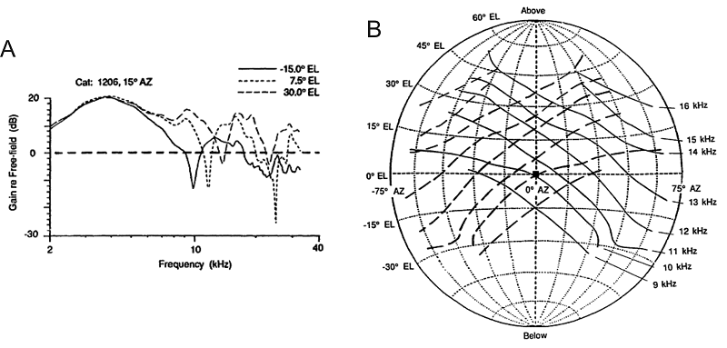
Figure 5.7
(A) Head-related
transfer functions of the cat for three sound source directions. Note the
prominent “first notch” at frequencies near 10 kHz. (B) Map of the frontal
hemifield of space, showing sound source directions associated with particular
first-notch frequencies. With the cat facing the coordinate system just as you
are, the solid diagonals connect all source directions associated with the
first-notch frequencies in the right ear (as indicated along the right margin).
Dashed lines show equivalent data for the left ear. Together, the first-notch
frequencies for the left and right ears form a grid of sound source direction
in the frontal hemifield.
From Rice et al.
(1992).
This grid of first-notch
frequencies thus provides a very neatly organized system for representing
spectral cues within the tonotopic organization of the DCN. Type IV neurons in
each DCN with inhibitory best frequencies between 9 and 15 kHz are “spatially
tuned” to broadband sound sources positioned along the diagonals shown in figure
5.7B, in the sense that these locations would maximally
suppress their high spontaneous firing. Combining this information from the two
nuclei on each side of the brainstem should then be sufficient to localize
broadband sources unambiguously in this region of space. There is certainly
evidence to support this. Bradford May and colleagues have shown that
localization accuracy by cats in the frontal sound field is disrupted if the
frequency range where the first notch occurs is omitted from the stimulus
(Huang & May, 1996), while cutting the fiber bundle known as the dorsal
acoustic stria, which connects the DCN to the inferior colliculus (IC), impairs
their ability to localize in elevation without affecting hearing sensitivity
(May, 2000).
It may have occurred to you that
cats and some other species can move their ears. This has the effect of
shifting the locations at which the spectral notches occur relative to the
head. Such movements are extremely useful for aligning sounds of interest with
the highly directional ears, so that they can be detected more easily. However,
ITDs are little affected by pinna movements, so it would appear that these
animals effectively perform their own cue trading experiments whenever the ears
move. Consequently, a continuously updated knowledge of pinna position is
required to maintain accurate sound localization. This is provided in the form
of somatosensory input to the DCN, which mostly originates from the muscle
receptors found in the pinna (Kanold & Young, 2001).
Although spectral notches are
undoubtedly important localization cues, psychophysical studies in humans
indicate that multiple spectral features contribute to sound localization
(Hofman & Van Opstal, 2002; Langendijk & Bronkhorst, 2002). Moreover,
nobody has documented an arrangement of HRTF notches or peaks in other
mammalian species that is as neat and orderly as that of the cat. This implies
that it is necessary to learn through experience to associate particular
spectral cues with a specific source direction. But even in the absence of a
systematic pattern, notch-sensitive type IV neurons in the DCN would still be
useful for detecting spectral cues and sending that information on to the
midbrain, and they are thought to serve this role not just in cats but in many
mammalian species.
5.3.2 Brainstem Encoding of Interaural-Level
Differences
As we have seen,
binaural cues provide the most important information for localization in the
horizontal plane. ILDs are perhaps the most familiar spatial cue to most of us
because we exploit them for stereophonic music. To measure these differences,
the brain must essentially subtract the signal received at one side from that
received at the other and see how much is left. Performing that subtraction
appears to be the job of a nucleus within the superior olivary complex known as
the lateral superior olive (LSO). The neural pathways leading to the LSO are
shown schematically in figure 5.8.
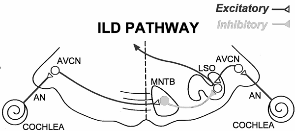
Figure 5.8
Schematic
of the ILD processing pathway in the auditory brainstem. AN, auditory nerve; AVCN,
anterior-ventral cochlear nucleus; MNTB, medial nucleus of the trapezoid body; LSO,
lateral superior olive.
Artwork by Prof. Tom Yin, reproduced with kind permission.
Since ILDs are high-frequency
sound localization cues, it is not surprising that neurons in the LSO, although
tonotopically organized, are biased toward high frequencies. These neurons are
excited by sound from the ipsilateral ear and inhibited by sound from the
contralateral ear; they are therefore often referred to as “IE” neurons. The
excitation arrives directly via connections from primary-like bushy cells in
the AVCN, while the inhibition comes from glycinergic projection neurons in the
medial nucleus of the trapezoid body (MNTB), which, in turn, receive their
input from globular bushy cells in the contralateral AVCN.
Given this balance of excitatory
and inhibitory inputs, an IE neuron in the LSO will not respond very strongly
to a sound coming from straight ahead, which would be of equal intensity in
both ears. But if the sound source moves to the ipsilateral side, the sound
intensity in the contralateral ear will decline due to the head shadowing
effects described earlier. This leads to lower firing rates in contralateral
AVCN neurons, and hence a reduction in inhibitory inputs to the LSO, so that
the responses of the LSO neurons become stronger. Conversely, if the sound moves to the contralateral side, the LSO receives less
excitation but stronger inhibition, and LSO neuron firing is suppressed. A
typical example of this type of ILD tuning in LSO neurons is shown in figure
5.9. In this manner, LSO neurons establish a sort of rate
coding for sound source location. The closer the sound source is to the
ipsilateral ear, the more strongly the neurons fire. Note that this rate code
is relatively insensitive to overall changes in sound intensity. If the sound
source does not move, but simply grows louder, then both the excitatory and the
inhibitory drives will increase, and their net effect is canceled out.
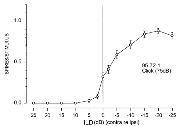
Figure 5.9
Firing
rate as a function of ILD for a neuron in the LSO of the rat.
Adapted from figure
2A of
IE neurons in the LSO are unusual
in that they prefer stimuli presented to the ipsilateral side. However, sensory
neurons in most brain areas tend to prefer stimulus locations on the opposite
side of the body. To make ILD-derived spatial sensitivity of LSO neurons
conform to the contralateral sensory representations found elsewhere, those
neurons send excitatory projections to the contralateral IC. Consequently, from
the midbrain onwards, central auditory neurons, just like those processing
touch or vision, will typically prefer stimuli presented in the contralateral
hemifield. The output from the LSO to the midbrain is not entirely crossed,
however, as a combination of excitatory and inhibitory projections also
terminate on the ipsilateral side (Glendenning et al., 1992). The presence of
ipsilateral inhibition from the LSO also contributes to the contralateral bias
in the spatial preferences of IC neurons.
5.3.3 Brainstem Encoding of Interaural
Time Differences
Although creating ILD
sensitivity in the LSO is quite straightforward, the processing of ITDs is
rather more involved and, to many researchers, still a
matter of some controversy. Clearly, to measure ITDs, the neural circuitry has
to somehow measure and compare the arrival time of the sound at each ear. That
is not a trivial task. Bear in mind that ITDs can be on the order of a few tens
of microseconds, so the arrival time measurements have to be very accurate. But
arrival times can be hard to pin down. Sounds may have gently ramped onsets,
which can make it hard to determine, with submillisecond precision, exactly
when they started. Even in the case of a sound with a very sharp onset, such as
an idealized click, arrival time measurements are less straightforward than you
might think. Recall from chapter 2 that the mechanical filters of the cochlea
will respond to click inputs by ringing with a characteristic impulse response
function, which is well approximated by a gamma tone. Thus, a click will cause
a brief sinusoidal oscillation in the basilar membrane (BM), where each segment
of the membrane vibrates at its own characteristic frequency. Hair cells
sitting on the BM will pick up these vibrations and stimulate auditory nerve
fibers, causing them to fire not one action potential, but several, and those
action potentials will tend to phase lock to the crest of the oscillations
(compare figures 2.4 and 2.12 in chapter 2).
Figure 5.10 illustrates this for BM segments
tuned to 1 kHz in both the left (shown in black) and right (shown in gray) ear,
when a click arrives in the left ear shortly before it arrives in the right.
The continuous lines show the BM vibrations, and the dots above the lines
symbolize the evoked action potentials that could, in principle, be produced in
the auditory nerve. Clearly, if the brain wants to determine the ITD of the
click stimulus that triggered these responses, it needs to measure the time
difference between the black and the gray dots. Thus, even if the sound stimuli
themselves are not sinusoidal, ITDs give rise to interaural phase differences.
To make ITD determination
possible, temporal features of the sound are first encoded as the phase-locked
discharges of auditory nerve fibers, which are tuned to relatively narrow
frequency bands. To a sharply tuned auditory nerve fiber, every sound looks
more or less like a sinusoid. In the example shown in figure
5.10, this phase encoding of the click stimulus brings
both advantages and disadvantages. An advantage is that we get “multiple looks”
at the stimulus because a single click produces regular trains of action
potentials in each auditory nerve. But there is also a potential downside. As
we pointed out in section 5.1, it may not be possible to determine from an
interaural phase difference which ear was stimulated first. Similarly, in the
case of figure 5.3, it is not necessarily
obvious to the brain whether the stimulus ITD corresponds to the distance from
a black dot to the next gray dot, or from a gray dot to the next black dot. To
you this may seem unambiguous if you look at the BM impulse functions in figure
5.3, but bear in mind that your auditory brainstem sees
only the dots, not the lines, and the firing of real auditory nerve fibers is
noisy, contains spontaneous as well as evoked spikes, and may not register some
of the basilar membrane oscillations because of the refractory period of the
action potential. Hence, some of the dots shown in the figure might be missing,
and additional, spurious points may be added. Under these, more realistic
circumstances, which interaural spike interval gives a correct estimate of the
ITD is not obvious. Thus, the system has to pool
information from several fibers, and is potentially vulnerable to phase
ambiguities even when the sounds to be localized are brief transients.
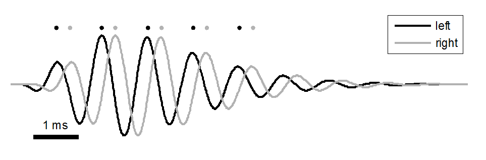
Figure 5.10
Basilar membrane
impulse responses in the cochlea of each ear to a click delivered with a small
interaural time difference.
The task of comparing the phases
in the left and right ear falls on neurons in the medial superior olive (MSO),
which, appropriately and in contrast to the LSO, is biased toward low
frequencies. As shown schematically in figure 5.11,
the MSO receives excitatory inputs from both ears (MSO neurons are therefore
termed “EE” cells) via monosynaptic connections from spherical bushy cells in
the AVCN. The wiring diagram in the figure is strikingly simple, and there seem
to be very good reasons for keeping this pathway as short and direct as
possible.
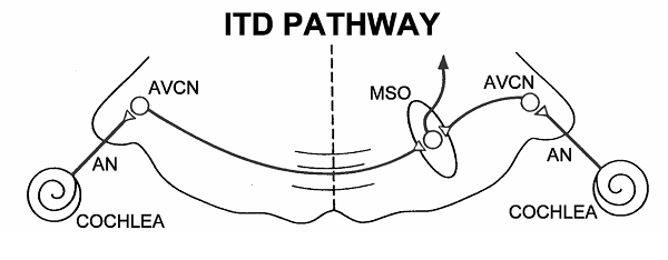
Figure 5.11
Connections
of the medial superior olive.
Artwork by Prof. Tom Yin, reproduced with kind permission.
Neurons in the central nervous
system usually communicate with each other through the release of chemical
neurotransmitters. This allows information to be combined and modulated as it
passes from one neuron to the next. But this method of processing comes at a
price: Synaptic potentials have time courses that are usually significantly
slower and more spread out in time than neural spikes, and the process of
transforming presynaptic spikes into postsynaptic potentials, only to convert
them back into postsynaptic spikes, can introduce noise, uncertainty, and
temporal jitter into the spike trains. Because ITDs are often very small,
indeed, the introduction of temporal jitter in the phase-locked spike trains
that travel along the ITD-processing pathway would be very bad news. To prevent
this, the projection from auditory nerve fibers to AVCN bushy cells operates
via unusually large and temporally precise synapses known as endbulbs of Held.
Although many convergent synaptic inputs in the central nervous system are normally
required to make a postsynaptic cell fire, a single presynaptic spike at an
endbulb of Held synapse is sufficient to trigger a spike in the postsynaptic
bushy cell. This guarantees that no spikes are lost from the firing pattern of
the auditory nerve afferents, and that phase-locked time structure information
is preserved. In fact, as figure 5.12 shows,
bushy cells respond to the sound stimulus with a temporal precision that is
greater than that of the auditory nerve fibers from which they derive their
inputs.
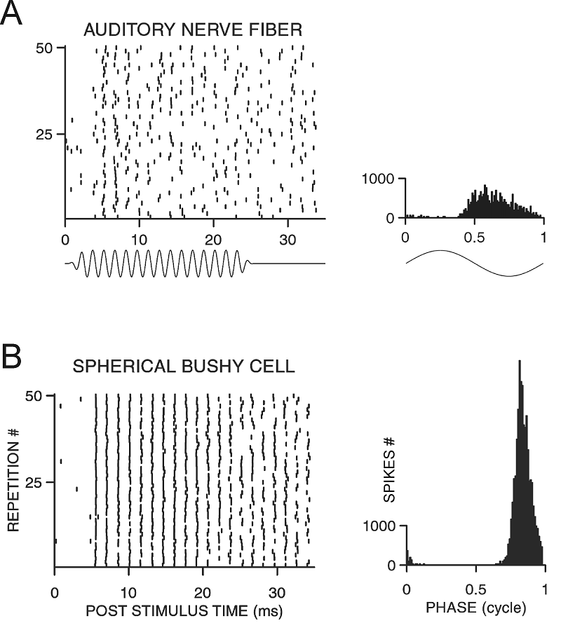
Figure 5.12
Phase-locked
discharges of an auditory nerve fiber (A) and a spherical bushy cell of the
AVCN (B). The plots to the left show individual responses in
dot raster format. Each dot represents the firing of an action
potential, with successive rows showing action potential trains to several
hundred repeat presentations of a pure-tone stimulus. The stimulus waveform is
shown below the raster plots. The histograms on the right summarize the
proportion of spikes that occurred at each phase of the stimulus. The bushy
cell responses are more reliable and more tightly clustered around a particular
stimulus phase than those of the auditory nerve fiber.
From Joris, Smith,
and Yin (1998).
AVCN bushy cells therefore supply
MSO neurons with inputs that are precisely locked to the temporal fine
structure of the sound in each ear. All the MSO neurons need to do to determine
the sound’s ITD is compare these patterns from the left and right ears. For a
long time, it has been thought that MSO neurons carry out this interaural
comparison by means of a delay line and coincidence detector arrangement, also
known as the Jeffress model (Jeffress, 1948). The idea behind the Jeffress
model is quite ingenious. Imagine a number of neurons lined up in a row, as
shown schematically in figure 5.13. The lines coming from
each side indicate that all five neurons shown receive inputs, via the AVCN,
from each ear. Now let us assume that the neurons fire only if the action potentials
from each side arrive at the same time, that is, the MSO neurons act as
“coincidence detectors.” However, the axons from the AVCN are arranged on each
side to form opposing “delay lines,” which results in the action potentials
arriving at each MSO neuron at slightly different times from the left and right
ears. Thus, for our hypothetical neuron A in figure 5.13,
the delay from the left ear is only 0.1 ms, while that from the right ear is
0.5 ms. For neuron B, the left ear delay has become a little longer (0.2 ms)
while that from the right ear is a little shorter (0.4 ms), and so on. These
varying delays could be introduced simply by varying the relative length of the
axonal connections from each side. But other factors may also contribute, such as
changes in myelination, which can slow down or speed up action potentials, or
even a slight “mistuning” of inputs from one ear relative to the other. Such
mistuning would cause small interaural differences in cochlear filter delays,
as we discussed in chapter 2 in the context of figures 2.4 and 2.5.
Figure 5.13
The
Jeffress delay-line and coincidence detector model.
Now let us imagine that a sound
comes from directly ahead. Its ITD is therefore zero, which will result in
synchronous patterns of discharge in bushy cells in the left and right AVCN.
The action potentials would then leave each AVCN at the same time, and would
coincide at neuron C, since the delay lines for that neuron are the same on
each side. None of the other neurons in figure 5.13
would be excited, because their inputs would arrive from each ear at slightly
different times. Consequently, only neuron C would respond vigorously to a
sound with zero ITD. On the other hand, if the sound source is positioned
slightly to the right, so that sound waves now arrive at the right ear 0.2 ms
earlier than those at the left, action potentials leaving from the right AVCN
will have a head start of 0.2 ms relative to those from left. The only way
these action potentials can arrive simultaneously at any of the neurons in figure
5.13 is if those coming from the right side are delayed so
as to cancel out that head start. This will happen at neuron B, because its
axonal delay is 0.2 ms longer from the right than from the left. Consequently,
this neuron will respond vigorously to a sound with a right ear–leading ITD of
0.2 ms, whereas the others will not. It perhaps at first seems a little
counterintuitive that neurons in the left MSO prefer sounds from the right, but
it does make sense if you think about it for a moment. If the sound arrives at
the right ear first, the only way of getting the action potentials to arrive at
the MSO neurons at the same time is to have a correspondingly shorter neural
transmission time from the left side, which will occur in the MSO on the left
side of the brain.
A consequence of this arrangement
is that each MSO neuron would have a preferred or best ITD, which varies
systematically to form a neural map or “place code.” All of our hypothetical
neurons in figure 5.13 would be tuned to the same
sound frequency, so that each responds to the same sound, but does so only when
that sound is associated with a particular ITD. This means that the full range
of ITDs would have to be represented in the form of the Jeffress model within
each frequency channel of the tonotopic map.
The Jeffress model is certainly an
attractive idea, but showing whether this is really how the MSO works has
turned out to be tricky. The MSO is a rather small nucleus buried deep in the
brainstem, which makes it difficult to study its physiology. However, early
recordings were in strikingly good agreement with the Jeffress model. For
example, Catherine Carr and Masakazu Konishi (1988) managed to record from the
axons from each cochlear nucleus as they pass through the nucleus laminaris, the
avian homolog of the MSO, of the barn owl. They found good anatomical and
physiological evidence that the afferent fibers act as delay lines in the
predicted fashion, thereby providing the basis for the topographic mapping of
ITDs. Shortly thereafter, Yin and Chan (1990) published recordings of cat MSO
neurons, which showed them to behave much like “cross-correlators,” implying
that they may also function much like coincidence detectors.
So what does it mean to say that
MSO neurons act like cross-correlators? Well, first of all let us make clear
that the schematic wiring diagrams in figures 5.11 and 5.13
are highly simplified, and may give the misleading impression that each MSO
neuron receives inputs from only one bushy cell axon from each AVCN. That is not
the case. MSO neurons have a distinctive bipolar morphology, with a dendrite
sticking out from either side of the cell body. Each dendrite receives synapses
from numerous bushy cell axons from either the left or right AVCN.
Consequently, on every cycle of the sound, the dendrites receive not one
presynaptic action potential, but a volley of many action potentials, and these
volleys will be phase locked, with a distribution over the cycle of the
stimulus much like the histogram shown on the bottom right of figure
5.12. These volleys will cause fluctuations in the
membrane potential of the MSO dendrites that look a lot like a sine wave, even
if the peak may be somewhat sharper, and the valley rather broader, than those
of an exact sine wave (Ashida et al., 2007). Clearly, these quasi-sinusoidal
membrane potential fluctuations in each of the dendrites will summate
maximally, and generate the highest spike rates in the MSO neuron, if the
inputs to each side are in phase.
Thus, an MSO neuron fires most
strongly if, after compensation for stimulus ITD through the delay lines
mentioned above, the phase delay between the inputs to
the dendrites is zero, plus or minus an integer number of periods of the
stimulus. Thus, as you can verify in figure 5.14,
an MSO neuron that responds strongly to a 250-Hz tone (i.e., a tone with a 4,000
μs long period) with an ITD of 600 μs will also respond strongly at
ITDs of 4,600 μs, or at -3,400 μs, although these “alternative best
ITDs” are too large to occur in nature. The output spike rates of MSO neurons
as a function of stimulus ITD bear more than a passing resemblance to the
function you would obtain if you used a computer to mimic cochlear filtering
with a bandpass filter and then calculated the cross-correlation of the filtered
signals from the left and right ears. (Bandpass filtering will make the stimuli
look approximately sinusoidal to the cross-correlator, and the
cross-correlation of two sinusoids that are matched in frequency is itself a
sinusoid.)
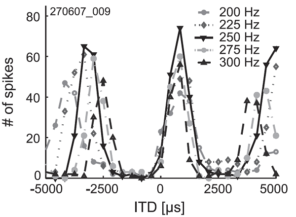
Figure 5.14
Spike rate of a neuron
in the MSO of a gerbil as a function of stimulus ITD. The stimuli were pure-tone
bursts with the frequencies shown.
From Pecka and
colleagues (2008).
A cross-correlator can be thought
of as a kind of coincidence detector, albeit not a very sharply tuned one. The
cross-correlation is large if the left and right ear inputs are well matched,
that is, if there are many temporally coincident spikes. But MSO neurons may
fire even if the synchrony of inputs from each ear is not very precise (in
fact, MSO neurons can sometimes even be driven by inputs from one ear alone).
Nevertheless, they do have a preferred interaural phase difference, and
assuming that phase ambiguities can be discounted, the preferred value should
correspond to a single preferred sound source direction relative to the
interaural axis, much as Jeffress envisaged.
The early experimental results,
particularly those from the barn owl, made many researchers in the field
comfortable with the idea that the Jeffress model was essentially correct, and
chances are you have read an account of this in a neuroscience textbook.
However, more recently, some researchers started having doubts that this
strategy operates universally. For example, McAlpine, Jiang, and Palmer (2001)
noticed that certain properties of the ITD tuning functions they recoded in the
inferior colliculus (IC) of the guinea pig appeared to be inconsistent with the
Jeffress model. Now the output from the MSO to the midbrain is predominantly
excitatory and ipsilateral. This contrasts with the mainly contralateral
excitatory projection from the LSO, but still contributes to the contralateral
representation of space in the midbrain, because, as we noted earlier, neurons
in each MSO are sensitive to ITDs favoring the opposite ear and therefore
respond best to sounds on that side. In view of this, McAlpine and colleagues
assumed that ITD tuning in the IC should largely reflect the output of MSO
neurons. They found that, for many neurons, the best ITDs had values so large
that a guinea pig, with its relatively small head, would never experience them
in nature (figure 5.15). If we assume that a
neuron’s best ITD is meant to signal a preferred sound source direction, then
it must follow that the neurons are effectively tuned to sound source
directions that do not exist.
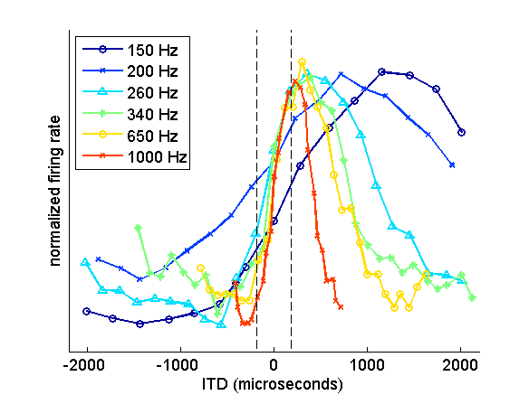
Figure 5.15
ITD tuning varies with
neural frequency sensitivity. Each function represents the ITD tuning of six
neurons recorded in the guinea pig inferior colliculus. Each neuron had a
different best frequency, as indicated by the values in the inset. Neurons with
high best frequencies have the sharpest ITD tuning functions, which peak close
to the physiological range (±180 µs), whereas neurons with lower best
frequencies have wider ITD functions, which peak at longer ITDs that are often
well outside the range that the animal would encounter naturally.
Adapted from
McAlpine (2005).
These authors also observed that
the peaks of the ITD tuning curves depend on each neuron’s preferred sound
frequency: The lower the best frequency, the larger the best ITD. That
observation, too, seems hard to reconcile with the idea that ITDs are
represented as a place code, because it means that ITDs should vary across
rather than within the tonotopic axis. The dependence of ITD tuning on the
frequency tuning of the neurons is easy to explain. As we have already said,
these neurons are actually tuned to interaural phase differences, so the longer
period of lower frequency sounds will result in binaural cross-correlation at
larger ITDs. You can see this in figure 5.14,
where successive peaks in the ITD tuning curve are spaced further apart at
lower frequencies, with their spacing corresponding to one stimulus period.
This also means that the ITD tuning curves become broader at lower frequencies
(figure 5.15), which does not seem
particularly useful for mammals that depend on ITDs for localizing
low-frequency sounds.
There is, however, another way of
looking at this. You can see in figure
5.15 that the steepest region of each of the ITD
tuning curves is found around the midline, and therefore within the range of
naturally encountered ITDs. This is the case irrespective of best frequency.
These neurons therefore fire at roughly half their maximal rate for sounds
coming from straight ahead, and respond more or less strongly depending on
whether the sound moves toward the contra- or ipsilateral side, respectively.
Such a rate code would represent source locations near the midline with great
accuracy, since small changes in ITD would cause relatively large changes in
firing rate. Indeed, this is the region of space where, for many species, sound
localization accuracy is at its best.
Studies of ITD coding in mammals
have also called another aspect of the Jeffress model into question. We have so
far assumed that coincidence detection in the MSO arises through simple
summation of excitatory inputs. However, in addition to the excitatory
connections shown in figure 5.11, the MSO, just like the LSO,
receives significant glycinergic inhibitory inputs from the MNTB and the
lateral nucleus of the trapezoid body. Furthermore, the synaptic connections to
the MNTB that drive this inhibitory input are formed by a further set of
unusually large and strong synapses, the so-called calyces of Held. It is
thought that these calyces, just like the endbulbs of Held that provide
synaptic input from auditory nerve fibers to the spherical bushy cells, ensure
high temporal precision in the transmission of signals from globular bushy cell
to MNTB neurons. As a result, inhibitory inputs to the MSO will also be
accurately phase locked to the temporal fine structure of the sound stimulus.
The Jeffress model has no apparent
need for precisely timed inhibition, and these inhibitory inputs to the MSO
have therefore often been ignored. But Brand and colleagues (2002) showed that
blocking these inhibitory inputs, by injecting tiny amounts of the glycinergic
antagonist strychnine into the MSO, can alter the ITD
tuning curves of MSO neurons, shifting their peaks from outside the
physiological range to values close to 0 µs. This implies that, without these
inhibitory inputs, there may be no interaural conduction delay. How exactly
these glycinergic inhibitory inputs influence ITD tuning in the MSO remains a
topic of active research, but their role can no longer be ignored.
Based on the ITD functions they
observed, McAlpine and colleagues proposed that it should be possible to
pinpoint the direction of the sound source by comparing the activity of the two
broadly tuned populations of neurons on either side of the brain. Thus, a
change in azimuthal position would be associated with an increase in the
activity of ITD-sensitive neurons in one MSO and a decrease in activity in the other.
This notion that sound source location could be extracted by comparing the
activity of neurons in different channels was actually first put forward by von
Békésy, whose better known observations of the mechanical tuning of the cochlea
are described in chapter 2. There is a problem with this, though. According to
that scheme, the specification of sound source direction is based on the
activity of neurons on both sides of the brain. It is, however, well
established that unilateral lesions from the midbrain upward result in
localization deficits that are restricted to the opposite side of space
(Jenkins & Masterton, 1982), implying that all the information needed to
localize a sound source is contained within each hemisphere.
In view of these findings, do we
have to rewrite the textbook descriptions of ITD coding, at least as far as
mammals are concerned? Well, not completely. In the barn owl, a bird of prey
that is studied intensively because its sound localization abilities are
exceptionally highly developed, the evidence for Jeffress-like ITD processing
is strong. This is in part due to the fact that barn owl auditory neurons are
able to phase lock, and thus to use ITDs, for frequencies as high as 9 kHz.
Interaural cross-correlation of sounds of high frequency, and therefore short
periods, will lead to steep ITD functions with sharp peaks that lie within the
range of values that these birds will encounter naturally. Consequently, a
place code arrangement as envisaged by Jeffress becomes an efficient way of
representing auditory space.
By contrast, in mammals, where the
phase locking limit is a more modest 3 to 4 kHz, the correspondingly shallower
and blunter ITD tuning curves will encode sound source direction most
efficiently if arranged to set up a rate code (Harper & McAlpine, 2004).
However, the chicken seems to have a Jeffress-like, topographic arrangement of
ITD tuning curves in its nucleus laminaris (Köppl & Carr, 2008). This is perhaps surprising since its neurons cannot phase lock, or
even respond, at the high frequencies used by barn owls, suggesting that
a rate-coding scheme ought to be more efficient given the natural range of ITDs
and audible sound frequencies in this species. Thus, there may be genuine and
important species differences in how ITDs are processed by birds and mammals,
perhaps reflecting constraints from evolutionary history as much as or more
than considerations of which arrangement would yield the most efficient neural
representation (Schnupp & Carr, 2009).
5.4 The Midbrain and Maps of Space
A number of brainstem
pathways, including those from the LSO, MSO, and DCN, converge in the IC and
particularly the central nucleus (ICC), which is its main subdivision. To a
large extent, the spatial sensitivity of IC neurons reflects the processing of
spatial cues that already took place earlier in the auditory pathway. But
brainstem nuclei also project to the nuclei of the lateral lemniscus, which, in
turn, send axons to the IC. Convergence of these various pathways therefore
provides a basis for further processing of auditory spatial information in the
IC. Anatomical studies carried out by Douglas Oliver and colleagues (Loftus et
al., 2004; Oliver et al., 1997) have shown that some of these inputs remain
segregated, whereas others overlap in the IC. In particular, the excitatory
projections from the LSO and MSO seem to be kept apart even for neurons in
these nuclei with overlapping frequency ranges. On the other hand, inputs from
the LSO and DCN converge, providing a basis for the merging of ILDs and
spectral cues, while the ipsilateral inhibitory projection from the LSO
overlaps with the excitatory MSO connections.
In keeping with the anatomy,
recording studies have shown that IC neurons are generally sensitive to more
than one localization cue. Steven Chase and Eric Young (2008) used virtual
space stimuli to estimate how informative the responses of individual neurons
in the cat IC are about different cues. You might think that it would be much
easier to combine estimates of sound source direction based on different
spatial cues if the cues are already encoded in the same manner. And as we saw
in the previous section, it looks as though the mammalian superior olivary
complex employs a rate code for both ITDs and ILDs. Chase and Young found,
however, that slightly different neural coding strategies are employed for
ITDs, ILDs, and spectral cues. ITDs are represented mainly by the firing rate
of the neurons, whereas the onset latencies and temporal discharge patterns of
the action potentials make a larger contribution to the coding of ILDs and
spectral notches. This suggests a way of combining the different sources of
information about the direction of a sound source, while at the same time
preserving independent representations of those cues. The significance of this
remains to be seen, but it is not hard to imagine that such a strategy could
provide the foundations for maintaining a stable spatial percept under
conditions where one of the cues becomes less reliable.
Another way of probing the
relevance of spatial processing in the IC is to determine how well the
sensitivity of the neurons found there can account for perceptual abilities.
Skottun and colleagues (2001) showed that the smallest detectable change in ITD
by neurons in the guinea pig IC matched the performance of human listeners.
There is also some evidence that the sensitivity of IC neurons to interaural
phase differences varies with the values to which they have recently been
exposed in ways that could give rise to sensitivity to stimulus motion (Spitzer
& Semple, 1998). This is not a property of MSO neurons and therefore seems
to represent a newly emergent feature of processing in the IC.
Earlier on in this chapter, we
drew parallels between the way sound source direction has to be computed within
the auditory system and the much more straightforward task of localizing
stimuli in the visual and somatosensory systems. Most of the brain areas
responsible for these senses contain maps of visual space or of the body
surface, allowing stimulus location to be specified by which neurons are
active. As we saw in the previous section, a place code for sound localization
is a key element of the Jeffress model of ITD processing, which does seem to
operate in the nucleus laminaris of birds, and barn owls in particular, even if
the evidence in mammals is much weaker.
The neural pathways responsible
for sound localization in barn owls have been worked out in considerable detail
by Masakazu Konishi, Eric Knudsen, and their colleagues. Barn owls are unusual
in that they use ITDs and ILDs for sound localization over the same range of
sound frequencies. Thus, the duplex theory does not apply. They also use these
binaural localization cues in different spatial dimensions. Localization in the
horizontal plane is achieved using ITDs alone, whereas ILDs provide the basis
for vertical localization. This is possible because barn owls have asymmetric
ears: The left ear opening within the ruff of feathers that surrounds the face
is positioned higher up on the head than the right ear opening. Together with
other differences between the left and right halves of the facial ruff, this
leads to the left ear being more sensitive to sounds originating from below the
head, while the right ear is more sensitive to sounds coming from above. The
resulting ILDs are processed in the posterior part of the dorsal lateral
lemniscal nucleus, where, like ITDs in the nucleus laminaris, they are
represented topographically (Manley, Koppl, & Konishi, 1988).
The ITD and ILD processing
pathways are brought together in the lateral shell of the central nucleus of
the IC. Because they use ITDs at such high frequencies, barn owls have a
particularly acute need to overcome potential phase ambiguities, which we discussed
in the context of figures 5.4 and 5.10 (Saberi et al.,
1999). The merging of information from different frequency channels is
therefore required to represent sound source location unambiguously. This
happens in the external nucleus of the IC, where the tonotopic organization
that characterizes earlier levels of the auditory pathway is replaced by a map
of auditory space (Knudsen & Konishi, 1978). In other words, neurons in
this part of the IC respond to restricted regions of space that vary in azimuth
and elevation with their location within the nucleus (figure
5.16). This is possible because the
neurons are tuned to particular combinations of ITDs and ILDs (Pena &
Konishi, 2002).
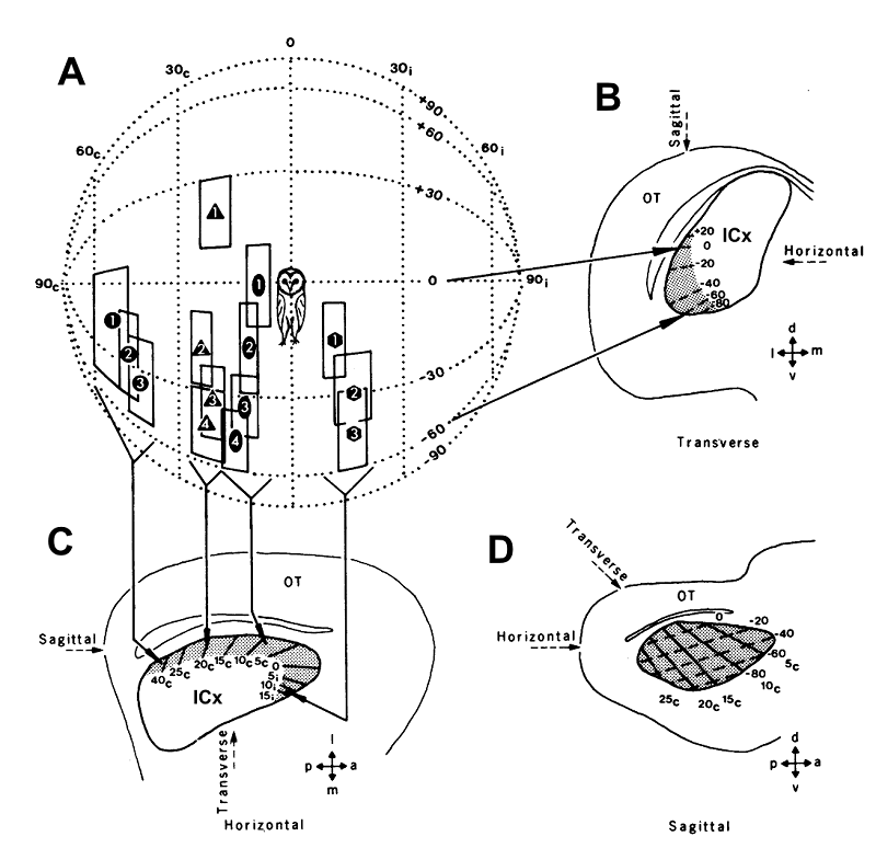
Figure 5.16
Topographic
representation of auditory space in the external nucleus of the inferior
colliculus of the barn owl. (A) The coordinates of the auditory “best areas” of fourteen different
neurons are plotted on an imaginary globe surrounding the animal’s head. (B) As
each electrode penetration was advanced dorsoventrally, the receptive fields of
successively recorded neurons gradually shifted downwards, as indicated on a
transverse section of the midbrain, in which isoelevation contours are depicted
by dashed lines within the ICX. (C) These neurons were recorded in four separate
electrode penetrations, whose locations are indicated on a horizontal section
of the midbrain. Note that the receptive fields shifted from in front of the
animal round to the contralateral side as the location of the recording
electrode was moved from the anterior to the posterior end of the ICX. This is
indicated by the solid lines within the ICX, which represent isoazimuth
contours. (D) The full map of auditory space can be visualized in a sagittal
section of the midbrain. The location of the optic tectum is indicated on each
section: a, anterior; p, posterior; d, dorsal; v, ventral; m, medial; l,
lateral.
From Knudsen and
Konishi (1978).
Constructing a map of the auditory
world may, on the face of it, seem like an effective way of representing the
whereabouts of sound sources within the brain, but it leaves open the question
of how that information is read out to control behavior. The key to this lies
in the next stage in the pathway. The external nucleus of the IC projects
topographically to the optic tectum, which also receives substantial visual
inputs. Knudsen (1982) demonstrated that auditory and visual inputs carrying
signals from the same regions in space converge onto single neurons in the
optic tectum. Thus, the tectum represents stimulus location independent of
whether that stimulus was heard or seen, and uses this information to guide
head-orienting behavior.
The discovery of a topographic
representation of auditory space in the midbrain of the barn owl led to
invigorated efforts to determine whether space maps are also present in the
mammalian auditory system. Palmer and King (1982) showed that this is the case
in the guinea pig superior colliculus (SC), the mammalian equivalent of the
barn owl’s optic tectum, and this has since been confirmed in other species.
Given the need to combine information across different frequencies to establish
a spatial topography, it should come as no surprise to learn that the mammalian
SC is not tonotopically organized. The acoustical basis for the space map in
mammals differs from that in owls, however, since this seems to rely
exclusively on ILDs and spectral cues (figure 5.17)
(Campbell et al., 2008; Palmer & King, 1985).
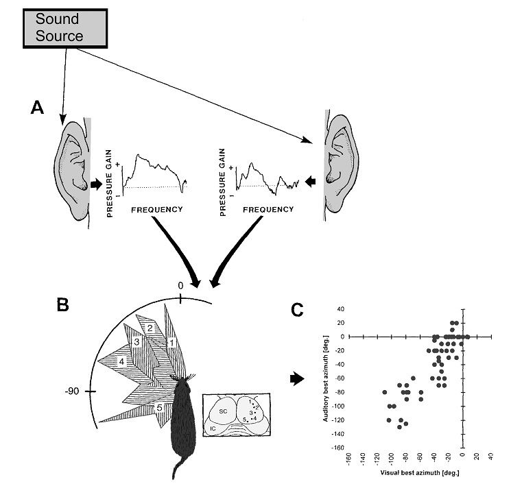
Figure 5.17
Representation
of auditory space in the mammalian superior colliculus (SC). (A) The spectral localization
cues generated by each external ear are shown for a sound source in the
anterior hemifield. Both ILDs and spectral cues are used in the synthesis of
the neural map of auditory space. (B) Spatial response profiles, plotted in
polar coordinates centered on the head, for different neurons recorded in the
right SC at the positions indicated by the corresponding numbers on the surface
view of the midbrain. Each response profile indicates how the action potential
firing rate varies with the azimuthal angle of the loudspeaker. Neurons in
rostral SC (recording site 1) respond best to sounds located in front of the
animal, whereas the preferred sound directions of neurons located at
progressively more caudal sites (1®5) shift systematically into the contralateral hemifield. IC, inferior colliculus. (C) Relationship between the visual
and auditory space maps in the ferret SC. For each vertical electrode
penetration, the auditory best azimuths (loudspeaker direction at which maximal
response was recorded) of neurons recorded in the intermediate and deep layers
of the SC are plotted against the corresponding visual coordinates of neurons
recorded in the overlying superficial layers. 0° refers to the anterior
midline, and negative numbers denote positions in the hemifield contralateral
to the recording site. A similar correspondence between the visual and auditory
maps is also found for stimulus elevation, which is mapped mediolaterally
across the surface of the SC.
Like the optic tectum in the barn
owl, the mammalian SC is a multisensory structure, and the auditory
representation is superimposed on maps of visual space and of the body surface
that are also present there. Indeed, one of the more striking features of the
auditory topography in different species is that the range of preferred sound
directions covaries with the extent of the visual map, as shown in figure
5.18 for the auditory and visual azimuth representations
in the ferret SC. These different sensory inputs are transformed by the SC into
motor commands for controlling orienting movements of the eyes, head, and, in
species where they are mobile, the external ears. Besides providing a common
framework for sensorimotor integration, aligning the different sensory inputs
allows interactions to take place between them, which give rise to enhanced
responses to stimuli that are presented in close temporal and spatial proximity
(Stein, Meredith, & Wallace, 1993).
Attractive though this arrangement
is, transforming auditory inputs into a format that is dictated by other
sensory modalities presents a new challenge. We have already seen that
estimates of current pinna position are required in cats to ensure that
movements of the ears do not result in conflicting information being provided
by different acoustic localization cues. But merging auditory and visual inputs
makes sense only if current eye position is also taken into account, so that the
accuracy of a gaze shift toward an auditory target will be preserved
irrespective of the initial position of the eyes. This is indeed the case in
the SC, where recordings in awake animals (Hartline et al., 1995; Jay & Sparks,
1984), and even in anesthetized animals who undergo passive eye displacement
(Zella et al., 2001), have shown that auditory responses can be modulated by
eye position; this indicates that, at least to some degree, auditory space is
represented there in eye-centered coordinates, rather than the purely
head-centered reference frame in which the localization cues are thought to be
initially encoded. What is more surprising, though, is that the activity of
neurons in tonotopically organized areas, including the IC (Groh et al., 2001)
and the auditory cortex (Werner-Reiss et al., 2003), can also change with gaze
direction.
5.5 What Does the Auditory Cortex Add?
Because many aspects
of auditory spatial perception can apparently be accounted for by the
substantial processing that takes place subcortically, it is tempting to
conclude that the process of sound localization is largely complete at the
level of the midbrain. This is not the end of the story, however, since we know
the auditory cortex also plays an essential part in supporting spatial
perception and behavior.
The clearest evidence for this
comes from the prominent localization deficits that result from ablating or
reversibly deactivating particular auditory cortical areas (Heffner & Heffner,
1990; Jenkins & Masterton, 1982; Lomber & Malhotra, 2008). In these
studies, the ability of animals to discriminate between or pick out the
location of sound sources on the opposite side of space is disrupted if the
cortex is silenced on one side. If both the left and right sides of the cortex
are affected, then the animals perform poorly on each side while retaining some
ability to distinguish between sound sources positioned on either side of the
midline. The deficits are most pronounced in species such as primates and
carnivores with a well-developed cortex, and are also seen in humans with
temporal lobe damage.In contrast to other species, however,
humans appear to show a right-hemisphere dominance for sound localization.
Thus, Zatorre and Penhune (2001) found that damage to the right auditory cortex
can impair spatial perception on both sides, whereas left-sided lesions may
have little effect on sound localization.
As with other aspects of auditory
perception, an important question in these studies is the relative involvement
of different cortical areas. Jenkins and Merzenich (1984) addressed this issue by
attempting to lesion the representation of a restricted band of frequencies in
A1 of the cat, leaving the rest of the cortex intact, or, conversely, by
destroying the whole of auditory cortex with the exception of a region of A1
that represented a narrow band of frequencies. They found that the small
lesions resulted in localization deficits that were specific to the sound
frequencies represented within the damaged area, whereas the larger lesions
impaired the localization of brief sounds at all frequencies except those
spared by the lesion.
While many other studies support
the conclusion that A1 is necessary for normal sound localization, it is no
longer possible to claim that this cortical area is sufficient. For one thing,
larger deficits are observed if aspiration lesions include surrounding areas as
well as A1 than if they are restricted to it. But more convincing are studies
in which specific cortical fields are temporarily deactivated. Using this
approach, Stephen Lomber and colleagues (Malhotra, Hall, & Lomber, 2004)
have shown that several cortical areas are involved in sound localization, whereas
others are not. In one of these experiments, Lomber and Malhotra (2008) found
that cooling the posterior auditory field produced a localization deficit in
cats, but had no effect on their ability to carry out an auditory pattern
discrimination task, whereas deactivation of the anterior auditory field
produced the opposite result (figure 5.18).
This suggests that a division of labor exists within the auditory cortex, with
different areas being responsible for the processing of spatial and nonspatial
information. But as we saw in chapters 3 and 4, this may have more to do with
where those areas project than with fundamental differences in the way they
process different types of sound.
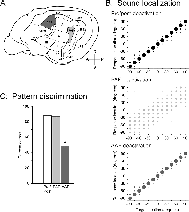
Figure 5.18
Behavioral
evidence for the involvement of separate cortical areas in spatial and nonspatial
auditory tasks.
(A) Lateral view of the left cerebral hemisphere of the cat showing the
auditory areas. AAF, anterior auditory field (dark gray); AI, primary auditory
cortex; AII, second auditory cortex; dPE, dorsal posterior ectosylvian area;
DZ, dorsal zone of auditory cortex; FAES, auditory field of the anterior
ectosylvian sulcus; IN, insular region; iPE, intermediate posterior ectosylvian
area; PAF, posterior auditory field (light gray); T, temporal region; VAF,
ventral auditory field; VPAF, ventral posterior auditory field; vPE, ventral
posterior ectosylvian area. Sulci (lowercase): aes, anterior ectosylvian; pes,
posterior ectosylvian; ss, suprasylvian. Other abbreviations: A, anterior; D,
dorsal; P, posterior; V, ventral. (B) Localization performance for one cat
before and following cooling deactivation (top panel), during bilateral cooling
of PAF cortex (middle panel) and during bilateral cooling of AAF cortex (bottom
panel). Target location is indicated on the x-axis and response location on the
y-axis. Area of the circle at each position indicates the percentage of
responses made to that location. (C) Mean temporal pattern discrimination
performance (mean ![]() s.e.m.)
for the same cat before and following cooling deactivation (pre, white), during
bilateral cooling of PAF cortex (light gray), and during bilateral cooling of
AAF cortex (dark gray).
s.e.m.)
for the same cat before and following cooling deactivation (pre, white), during
bilateral cooling of PAF cortex (light gray), and during bilateral cooling of
AAF cortex (dark gray).
These experiments clearly
establish that the auditory cortex plays an essential role in spatial hearing.
But how is sound source location represented there? As in other brain regions,
the spatial receptive fields of cortical neurons have been mapped out by
recording the spiking activity of neurons in response to sounds delivered from
free-field loudspeakers positioned around the head. These showed that cortical
receptive fields vary in size both from one neuron to another and with the type
of stimulus used, and they generally expand as the sound level is increased
(Middlebrooks & Pettigrew, 1981; Rajan et al., 1990; Woods et al., 2006).
In keeping with the behavioral deficits produced by ablation or deactivation of
the auditory cortex in one hemisphere, the receptive fields of most cortical
neurons are found on the contralateral side of the animal, although some
neurons prefer sound sources near the frontal midline or on the ipsilateral
side. Studies using virtual space stimuli allow the stimulus location to be
changed digitally over headphones and can therefore provide a more detailed
characterization of the receptive fields. This approach has confirmed that
cortical receptive fields can be quite heterogeneous (figure
5.19), although the majority are broadly tuned to the
contralateral hemifield.
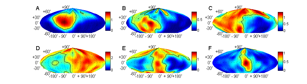
Figure 5.19
Six examples of
spatial receptive fields measured in the primary auditory cortex of the ferret
using virtual acoustic space stimuli derived from acoustical measurements of
the animals’ own ears’ SRFs.
From Mrsic-Flogel,
King, and Schnupp (2005).
We have already seen that
different localization cues can be combined by individual neurons in the IC.
Insofar as those neurons contribute to the ascending pathways, this must be the
case for the cortex, too. As in subcortical nuclei, low-frequency cortical
neurons are sensitive to ITDs, whereas high-frequency neurons rely more on
ILDs. But spectral cues generated by the filter properties of the external ear also
contribute. Thus, at near-threshold sound levels, high-frequency A1 neurons
have “axial” receptive fields that are centered on the acoustical axis of the
contralateral ear. This is the region where the acoustical gain is at its
maximum, indicating that the receptive fields of the neurons are shaped by
pinna directionality. As for the study of subcortical stations, in cortex the
use of virtual acoustic space techniques has also proved very valuable, making
it possible to map out spatial receptive field properties of cortical neurons
in great detail (Brugge et al., 2001) and even to chart their spatiotemporal
receptive fields (Jenison et al., 2001). Furthermore, substituting spectral
cues to make one animal listen through the “virtual ears” of another
changes cortical spatial receptive field properties (Mrsic-Flogel et al.,
2001). Schnupp and colleagues (2001) extended this study to show that, in many
cases, the location and shape of the spatial receptive fields of neurons in
ferret A1 can be explained by a linear combination of their frequency
sensitivity to stimulation of each ear and the directional properties of the
auditory periphery (figure 5.20). This linear estimation
model can also account for the way receptive fields change with increasing
sound level, although it works better for neurons that receive predominantly
excitatory inputs from the contralateral ear and inhibitory inputs from the
ipsilateral ear, and are therefore sensitive to ILDs, than to those receiving
excitatory binaural inputs and are likely to be sensitive to ITDs (Mrsic-Flogel
et al., 2005). Intriguingly, it also predicts changes in the spatial receptive
field caused by “listening through foreign virtual ears,” and it can predict
the observed improvement in spatial sensitivity seen with age as the head and
ears grow (Mrsic-Flogel, Schnupp, & King, 2003), a finding that we shall
return to in chapter 7.
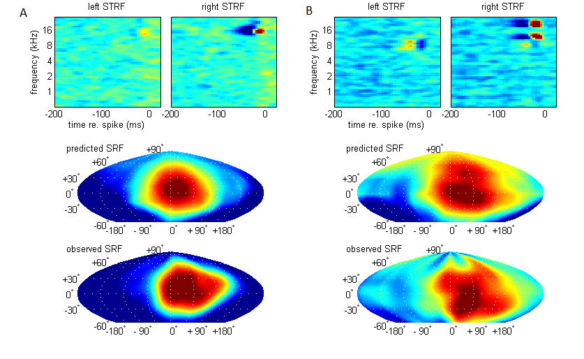
Figure 5.20
Predicting
spatial responses from the frequency tuning of two different neurons (A, B) in
ferret A1. The
upper plots show the spectrotemporal receptive fields (STRFs) measured by
reverse correlation to random chord stimuli for each ear. Each STRF was convolved
with the energy spectrum vectors of virtual space stimuli presented to that ear
for different virtual sound directions, and used to predict the SRFs of the
neuron (middle row). Comparison with the observed STRF (bottom row) reveals a
close fit between the two.
From Schnupp,
Mrsic-Flogel, and King (2001).
Early studies of the binaural
sensitivity of A1 neurons suggested that EI and EE neurons are arranged in a
series of bands that run orthogonal to the tonotopic axis, giving rise to the
notion that A1 may possess a series of intertwined maps of different sound
features, not unlike the regular organization of stimulus preferences in the
visual cortex. As binaural response properties have been classified in greater
detail, however, it has become clear that there is nothing more than a local
clustering of neurons with similar response properties (Nakamoto, Zhang, &
Kitzes, 2004; Rutkowski et al., 2000). This is also the case for the spatial
receptive fields (Middlebrooks & Pettigrew, 1981; Rajan et al., 1990). As
you can see in figure 5.21,
the spatial sensitivity of cortical neurons can vary from one side of the
midline to the other, indicating marked differences in their sensitivity to
different localization cues, but there is no evidence for a map of auditory
space in the cortex equivalent to that seen in the SC or to the maps of
stimulus location that characterize the visual and somatosensory cortices.
Given the importance of the
auditory cortex in sound localization, you might find this surprising. It is
clearly possible to construct a map of auditory space in the brain, as studies
of the SC and parts of the IC have shown, but we have to be clear about how
that information is used. In the SC, auditory, visual, and somatosensory inputs
combine to guide reflexive orienting movements. That is clearly a key function
of the ability to determine the whereabouts of objects of interest in the
world, but processing in the auditory cortex is responsible for much more,
underlying our perception of what the sound source is in addition to where it
is located.
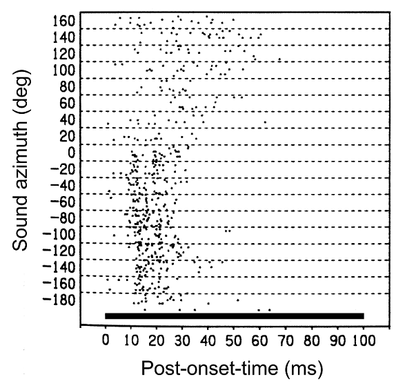
Figure 5.21
Auditory spatial
information carried by temporal spike patterns. Responses of a neuron in the
cat cortical anterior ectosylvian area to 100-ms noise bursts presented from
various azimuthal positions, as indicated along the y-axis. The dots indicate
the timing of action potential discharges. Each row of dots shows the temporal
discharge pattern evoked by one stimulus presentation. Repeated presentations are
shown in consecutive rows. Although individual responses are highly variable,
one can nevertheless observe a systematic change in the temporal firing pattern
as the sound source azimuth moves from the ipsilateral to the contralateral
side.
Adapted from Middlebrooks
et al. (1998).
We saw in the previous section
that IC neurons can carry spatial information not just in their firing rates,
but also in the timing of their action potentials. The potential importance of
spike timing has been investigated extensively in the cortex. As the example in
figure 5.22 shows, first-spike latencies tend to
vary inversely with spike counts, with sounds at the more effective stimulus
locations evoking more spikes with shorter latencies. However, temporal
discharge patterns can be modulated across the receptive field independently of
changes in firing rate, and a number of studies have shown that spike timing
can carry as much or even more information about sound-source location than
firing rate (Brugge, Reale, & Hind, 1996; Middlebrooks et al., 1998; Nelken
et al., 2005). Indeed,
As we have already stated, the
impact of cortical deactivation on sound localization depends on which areas
are silenced. There is also evidence in human imaging studies that the areas
that show the greatest changes in blood oxygenation when subjects are asked to
perform localization tasks are different from those engaged during sound
recognition tasks (Alain et al., 2001; Barrett & Hall, 2006; Maeder et al.,
2001). But recording studies have failed to reveal the clear division of labor
that these imaging results might imply, since some sensitivity to sound source
location is a property of all areas that have been investigated. Of course, that
is not particularly surprising in view of the extensive subcortical processing
of spatial information. Nevertheless, differences in spatial sensitivity have
been observed. Thus, in monkeys, neurons in caudal auditory cortical areas are
more sharply tuned for sound source location, and show a closer match to the
ability of the animals to detect a change in sound direction, than those in
core or rostral fields (Woods et al., 2006) (figure 5.22).
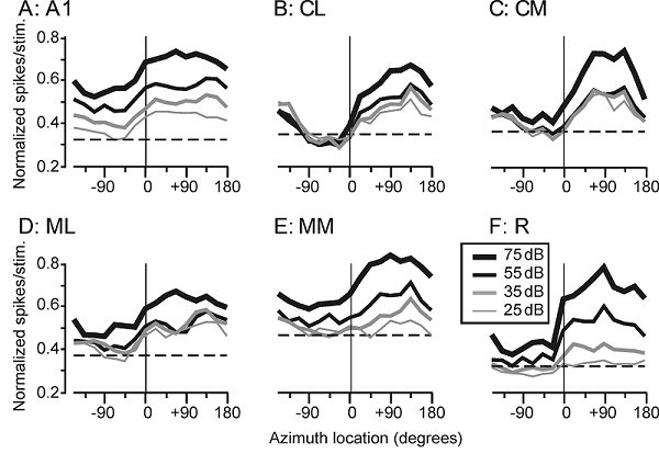
Figure 5.22
Normalized
distribution of activity as a function of stimulus level and azimuth recorded
in different areas of the monkey auditory cortex. Line thickness and shading
corresponds to the different levels (see inset in F). The horizontal dashed
line is the normalized spontaneous activity. Overall, the activity increased
with increasing stimulus levels and was more sharply tuned for the caudal belt
fields. From Woods et al. (2006).
Regional differences are also
found in cats. We saw in figure 5.18
that localization responses are impaired if posterior auditory field (PAF) is
silenced, whereas this is not the case if anterior auditory field (AAF) is
deactivated instead. Consistent with this, both the spike counts and
first-spike latencies of neurons in PAF are more strongly modulated by changes
in stimulus location and less affected by changes in sound level than those in
AAF. On the other hand, as we pointed out in chapter 4, it is likely that most
cortical neurons are sensitive to both spatial and nonspatial sound attributes
(Bizley et al.. 2009), so these represent quantitative
rather than qualitative differences in the preferences of the cortical neurons.
Although the spatial receptive
fields of cortical neurons tend to be very large in relation to behavioral
measures of spatial acuity, this does provide a means by which individual
neurons can convey spatial information in their spike discharge patterns across
a large range of stimulus locations. Based on responses like the one
illustrated in figure 5.21, Middlebrooks and
colleagues (1998) showed that computer-based classifiers can estimate sound source
location from the firing patterns of individual neurons. However, the accuracy
with which they do so is insufficient to account for sound localization
behavior. Consequently, attention has switched to the role of population coding
schemes, based on either the full spike discharge patterns (Stecker & Middlebrooks,
2003) or just the spike firing rates (Miller & Recanzone, 2009) or spike
latencies (Reale, Jenison, & Brugge, 2003). These population codes tend to
match behavioral performance more closely than those based on the response of
individual neurons.
We saw in section 5.3 that one
school of thought is that sound direction based on ITDs might be extracted by
comparing activity in the left and right MSOs. We also pointed out that this
scheme is not readily compatible with the localization deficits incurred when
auditory cortical areas are lesioned or inactivated on one side of the brain
only. But while most cortical neurons respond preferentially to sounds located
in the contralateral hemifield, others have ipsilateral receptive fields. This
led Stecker and colleagues (2005) to propose that sound localization might be
based on a comparison between the activity of populations of contralateral and
ipsilateral neurons within each
hemisphere. Although this has the attraction of embracing several of the ideas we
have described in this chapter,how auditory space is
represented in the cortex has yet to be fully established.
5.6 Localization in More Complex Environments
We have so far
considered sound localization in the simple and rather artificial situation in
which there is only one source. The reason for this is straightforward—the vast
majority of studies have been done that way. Moreover, in order to exclude
reflected sounds, psychophysical and recording experiments tend to be carried
out in anechoic chambers. A more natural situation would be one where multiple
sound sources are present at the same time in an environment with lots of room
reflections and echoes. Instead of having a single source, the reflected sound
waves will reach the listener from multiple directions, thereby distorting the
spatial cues associated with the direct sound. In fact, in many modern
environments such as a typical office or bedroom, the portion of the sound
energy that we receive indirectly as echoes from walls and ceiling can be
substantially greater than the direct sound.
In spite of this, human listeners
are normally entirely unaware of the “reflected sound images” that each echoic
surface creates, nor do these images seem to confuse or impair the accuracy of
the localization of the true source as much as might be expected. The critical
factor here seems to be that the reflected sound waves arrive at the ears
slightly later than the direct sound. The simplest way of demonstrating this is
to present a pair of brief sounds from two locations in space. For short
interstimulus delays of up to about 1 ms, the two
sounds are fused by the auditory system, and their perceived location lies
between the two source locations. This is known as “summing localization.” At
slightly longer delays, a single sound is still heard, but the second, or
lagging, sound is suppressed and the perceived location is dominated by the
actual location of the first sound. This is known as the “precedence effect”
(Wallach, Newman, & Rosenzweig, 1949). But if the lagging sound arrives
more than about 10 ms after the leading sound, the precedence effect breaks
down, and two separate sounds are heard, each close to its true location.
Neural correlates of the precedence effect have been described at various
stages of the central auditory pathway (Fitzpatrick et al., 1999; Litovsky,
1998; Mickey & Middlebrooks, 2005). However, neural responses to the
lagging sound tend to be suppressed in the cortex to longer delays than the
precedence effect persists for in humans, and modeling studies suggest that
much of this phenomenon can be accounted for by peripheral filtering together
with compression and adaptation in the responses of the cochlear hair cells
(Hartung & Trahiotis, 2001).
While the precedence effect
describes what happens when a single echo is simulated, this is still a far cry
from the more realistic situation in which sound waves traveling from a source
are reflected many times by objects in the environment, and therefore arrive at
the listener’s ears over a protracted period of time. Devore and colleagues
(2009) showed that reverberation affects the ITD sensitivity of IC neurons and
lateralization judgments by human listeners in a similar fashion. They found
that the spatial sensitivity of the neurons is better near the start of a
reverberant stimulus and degrades over time, which is consistent with the
gradual build up of reverberant energy as more and more reflections are
generated.
Binaural processing is important
not only for localizing sounds, but also for improving the detection of signals
against a background of interfering noise (Blauert, 1997). Imagine that you are
in a busy restaurant and trying to keep up with a particularly interesting
conversation while other people are speaking at the same time. If you block one
ear, this task becomes much harder. This is because binaural stimulation
results in less masking of the sound source of interest by the “noise”
emanating from other directions. Consequently, this important phenomenon is
often referred to as the “cocktail party effect.” It can be studied in the free
field and over headphones, but the classical paradigm involves the presentation
of a signal, usually a low-frequency tone, together with an interfering noise
to both ears. Inverting the phase of either the signal or the noise can result
in a 12- to 15-dB improvement in signal detection, a measure known as the
binaural masking level difference (BMLD) (Licklider, 1948). More ecologically
valid free-field studies, in which signal detection thresholds are measured
when the signal and masker are spatially separated, have obtained similar
levels of unmasking in both humans (Saberi et al., 1991) and ferrets (Hine,
Martin, & Moore, 1994). Although concerned more with stimulus detection
than localization, the responses of IC neurons to BMLD stimuli (Jiang,
McAlpine, & Palmer, 1997) are consistent with their ITD sensitivity to
tones and noise and with the results of human psychophysical studies.
In addition to considering how
spatial hearing is affected in the presence of multiple sound sources, we also
need to bear in mind that real objects very often stimulate more than one of
the senses. Just as we saw in chapter 4 in the context of speech perception,
visual cues can have a profound effect on sound localization. Thus,
localization accuracy can improve if the source is also visible to the subject
(Shelton & Searle, 1980; Stein, Huneycutt, & Meredith, 1988). On the
other hand, the presence of a synchronous visual stimulus that is displaced
slightly to one side of the auditory target can “capture” the perceived
location of the sound source, causing it to be mislocalized (Bertelson & Radeau,
1981) . This interaction between the senses provides
the basis for the ventriloquist’s illusion, and also explains why we readily
link sounds with their corresponding visual events on a television or movie
theater screen, rather than with the loudspeakers to one side. How vision
exerts these effects at the neuronal level is not understood, but we now know
that some neurons in the auditory cortex, as well as certain subcortical areas,
are also sensitive to visual or tactile stimulation. Indeed, Bizley and King
(2009) showed that visual inputs can sharpen the spatial sensitivity of
auditory cortical neurons, highlighting the importance of nonacoustic factors
in the neural representation of sound source location.