4
Hearing Speech
- 4.1 Speech as a Dynamic Stimulus
- 4.2 Categorical Perception of Speech Sounds
- 4.3 Subcortical Representations of Speech Sounds and Vocalizations
- 4.4 Cortical Areas Involved in Speech Processing: An Overview
- 4.5 The Role of Auditory Cortex: Insights from Clinical Observations
- 4.6 The Representation of Speech and Vocalizations in Primary Auditory Cortex
- 4.7 Processing of Speech and Vocalizations in Higher-Order Cortical Fields
- 4.8 Visual Influences
- 4.9 Summary
How our auditory
system supports our ability to understand speech is without a doubt one of the
most important aspects of hearing research. Severe hearing loss often brings social
isolation, particularly in those who were not born into deaf communities. For
most of us, the spoken word remains the primary communication channel,
particularly for the intimate, face-to-face exchanges and conversations that we
value so much. Naturally, we hope that, in due course, a better understanding
of the neurobiology of speech processing will improve our ability to repair
problems if this system goes wrong, or may allow us to build artificial speech
recognition systems that actually work, computers that we could actually talk
to. But while the potential rewards of research into the auditory processing of
speech are great, considerable technical and conceptual challenges also slow progress
in this area.
One major challenge stems from the
great complexity of speech. Essentially, a relatively modest number of speech
sounds (sometimes called “phones”) are recombined according to rules of
morphology to form words, and the words are recombined according to the rules
of grammar to form sentences. Our auditory brain can analyze the sound of any
sentence in a language we have learned, and decipher its meaning, yet the
number of correct, meaningful sentences in any language is so large as to be,
for all practical intents and purposes, infinite. Thus, when we learn a
language, we must not only acquire a sizeable lexicon of sound to meaning
mappings, but also perfect our grasp of the rules of morphology and grammar,
which allow us to manipulate and recombine the speech sounds to generate
endless varieties of new meanings.
Many animal species use
vocalizations to communicate with members of their own species, and sometimes
these communication sounds can be quite elaborate—consider, for example,
certain types of bird song, or the song of humpback whales. Nevertheless, the
complexity of human speech is thought to have no equal in the animal kingdom.
Dogs and some other domestic animals can be trained to understand a variety of
human vocal commands, and rhesus monkeys in the wild are thought to use between
thirty and fifty types of vocalization sounds to convey different meanings. The
number of different vocalizations used in these examples of
inter- and intraspecies vocal communication
is, however, fairly modest compared to the size of a typical human language
vocabulary, which can comprise tens of thousand words.
Animals also seem to have only a
limited capacity for recombining communication sounds to express new concepts
or describe their relationships. Even the most monosyllabic of human teenagers
readily appreciates that the meaning of the sentence “John eats and then flies” is very different from that of “And then John eats flies,” even though
in both sentences the speech sounds are identical and only their order has
changed a bit. Human children seem to learn such distinctions with little
effort. But while you do not need to explain this difference to your child, you
would have a terribly hard time trying to explain it to your dog. Indeed, many
language researchers believe that humans must have an innate facility for
learning and understanding grammar, which other animals seem to lack (Pinker,
1994).
Given this uniquely high level of
development of speech and language in humans, some may argue that there is
little point in studying the neural processing of speech and speechlike sounds in nonhuman animals. However, the tools
available to study the neural processing of communication sounds in humans are
very limited. Work with humans depends heavily either
on lesion studies that attempt to correlate damage to particular brain areas
with loss of function, on noninvasive functional imaging techniques, or on the
rare opportunities where electrophysiological recording or stimulation
experiments can be incorporated into open brain surgery for the treatment of
epilepsy. Each of these methods has severe limitations, and the level of detail
that is revealed by microelectrode recordings in animal brains is, as we shall
see, still an invaluable source of complementary information.
But using animal experiments to
shed light on the processing of vocalizations is not merely a case of “looking
for the key where the light is.” Human speech almost certainly evolved from the
vocal communication system of our primate ancestors, and it evolved its great
level of complexity in what is, in evolutionary terms, a rather short period of
time. No one is quite certain when humans started to speak properly, but we
diverged from the other surviving great ape species some 5 million years ago,
and our brains reached their current brain size some 1 to 2 million years ago (no
more than 100,000 generations). During this period, human speech circuits almost
certainly arose as an adaptation and extension of a more or less generic,
rudimentary mammalian vocal communication system, and animal experiments can
teach us a great deal about these fundamental levels of vocalization
processing.
Speech can be studied on many levels,
from the auditory phonetic level, which considers the manner in which
individual speech sounds are produced or received, to the syntactic, which considers
the role of complex grammatical rules in interpreting speech, or the semantic,
which asks how speech sounds are “mapped onto a particular meaning.” As we have
seen, studies of animal brains are unlikely to offer deep parallels or insights
into syntactic processing in the human auditory system, but neural
representations of speech sounds or animal vocalizations on the auditory/phonetic
level are bound to be very similar from one mammal to the next. Most mammals
vocalize, and do so in much the same way as we do (Fitch, 2006). As we briefly
described in section 1.6, mammals vocalize by pushing air through their larynx,
causing their vocal folds to vibrate. The resulting sound is then filtered
through resonant cavities in their vocal tracts, to impart on it a
characteristic “formant” structure. (On the book’s web site you can find short video clips showing
the human vocal folds and vocal tract in action. <flag>) There are some
differences in detail, for example, humans have a relatively deep-sitting
larynx, which makes for a particularly long vocal tract, and may allow us to be
a “particularly articulate mammal” (Ghazanfar & Rendall, 2008), but the basic layout is essentially the
same in all mammals, and the sounds generated by the vocal tracts of different
types of mammals consequently also have much in common. These similarities are more
obvious in some cases than in others (few humans, for example, would be very
flattered to hear that they sound like a donkey), but at times they can be very
striking, as in the case of Hoover the talking harbor seal.
When vocalizing to communicate
with each other, animals also face some of the same challenges we humans have
to overcome to understand speech. For example, both human and animal
vocalizations are subject to a fair amount of individual variability. No two
humans pronounce the same word absolutely identically. Differences in gender,
body size, emotional affect, as well as regional accents can all change the
sound of a spoken word without necessarily changing its meaning. Similarly,
dogs who differ in size or breed can produce rather
different sounding barks, yet despite these differences they all remain
unmistakably dog barks. Even song birds appear to have pronounced “regional dialects”
in their songs (Marler and Tamura, 1962). One common
problem in the processing of human speech as well as in animal vocalizations is
therefore how to correctly identify vocalizations, despite the often very
considerable individual variability. The neural processes involved in
recognizing communication sounds cannot be simple, low-level feature
extractors, but must be sophisticated and flexible pattern classifiers. We
still have only a very limited understanding of how animal and human brains
solve this kind of problem, but in experimental animals, unlike in humans,
these questions are at least in principle amenable to detailed experimental
observation.
This chapter is subdivided into
seven sections. In the first two sections, we examine the acoustic properties
of speech in greater detail, consider how the acoustic
features of speech evolve in time, and how they are categorized into distinct
speech sounds. In the third section, we describe how speech sounds are thought
to be encoded in subcortical structures. Our
knowledge of these subcortical representations comes
exclusively from animal experiments. In the fourth part, we briefly review the
anatomy of the cortex, and in the fifth we summarize what clinical observations
have taught us about the role played by various parts of the human cerebral
cortex in speech processing. In the last two sections, we examine the roles of
primary and higher-order cortical fields in greater detail, in the light of
additional information from human brain imaging and animal experiments.
4.1 Speech as a Dynamic Stimulus
When one considers
speech as an auditory stimulus, one obvious question to ask is: Is speech
radically different from other sounds, and if so, in what way? In section 1.6,
we looked at the production of vocalization sounds, and we noted that the
physics of vocal sound production is not particularly unusual, and contains
nothing that might not have an equivalent in the inanimate world. (You may wish
to glance through section 1.6 quickly before you read on if it is not fresh in
your mind.) The harmonics in voiced speech sounds produced by the oscillating
vocal folds are not so different from harmonics that might be produced by
vibrating taut strings or reeds. Unvoiced fricatives are caused by turbulent
airflow through constrictions in the vocal tract, and they resemble the noises
caused by rushing wind or water in both the way they are created and the way
they sound. Resonant cavities in our vocal tract create the all-important formants
by enhancing some frequencies and attenuating others, but they operate just
like any other partly enclosed, air-filled resonance chamber. So if speech
sounds are, in many respects, fundamentally similar to other environmental sounds
and noises, we might also expect them to be encoded and processed in just the
same way as any other sound would be by neurons of the auditory system.
Nevertheless, listeners only
rarely mistake other environmental sounds for speech, so perhaps there is
something about speech that makes it characteristically speechlike,
even if it is not immediately obvious what this something is. Consider the
sound of wind rushing through some trees. It may contain noisy hissing sounds that
resemble fricative consonants (fffff-, sss-, shhh-like sounds), and it
may also contain more harmonic, vaguely vowel-like “howling.” But the pitch and
amplitude contours of these sounds of howling wind usually change only slowly,
much more slowly than they would in speech. Meanwhile, a small stream of water
dropping into a pond might trickle, gurgle, and splash with an irregular rhythm
rather faster than that of speech. Thus, it seems that speech has its own
characteristic rhythm. Speech sounds change constantly in a manner that is
fast, but not too fast, and somewhat unpredictable yet not entirely irregular.
But can we turn this intuition regarding possible characteristic rhythms of
speech into something more tangible, more quantifiable?
One way to approach this question
is to consider the mechanisms of speech production in a little more detail. A
good example of this type of analysis can be found in a paper by Steven
Greenberg (2006), in which he argues that the syllable may the most appropriate
unit of analysis for speech sounds. Based on a statistical analysis of a corpus
of spoken American English, he concluded that syllables consist of an optional
“onset” (containing between zero and three consonants), an obligatory “nucleus”
(a vowel sound, which can be either a monophthong
like the /a/ in “at,” or a diphthong, like the /ay/ in “may”), and an optional
“coda” (containing between zero and four consonants). A single English syllable
can therefore be as simple as “a” or as elaborate as “straights.” Greenberg
would argue that more “atomic” speech sound units, such as the phoneme, or
phone, are unreal in the sense that they have no independent existence outside
the syllabic framework. Furthermore, he points out that the information content
of consonants depends on the syllabic context. For example, onsets are more
informative than codas, as can be seen by the fact that consonants in the coda
can often be lost without any loss of intelligibility (consider the lost /d/ in
“apples an’ bananas”). Given the diversity of English syllables, it is
unsurprising that they can also vary considerably in their temporal extent.
English syllables are typically 100 to 500 ms long, and are characterized by an
“energy arc,” since the vowel nucleus is normally up to 40 dB more intense than
the consonants of the onset or the coda. Note that not all languages exhibit as
much phonetic diversity in their syllables as English. In spoken Japanese, for
example, onsets very rarely comprise more than a single consonant, and the only
commonly used coda to a syllable is an optional “n.” Consequently, in Japanese
there are only a few hundred possible syllables, while in English there are
many thousands, but the onset-nucleus-coda syllabic structure is clearly a
feature of both languages.
As mentioned in chapter 1,
engineers like to refer to changes in a signal over time as “modulations”, and
they distinguish two fundamental types: amplitude modulation (AM, meaning the
sound gets louder or quieter) and frequency modulation (FM, meaning the
frequency content of the sound changes). Greenberg’s observation of one energy
arc in every spoken syllable, and one syllable every few hundreds of milliseconds
or so would lead us to expect that speech sounds should exhibit marked AM at
modulation rates of a few Hertz. Is this expectation borne out? If you look at
spectrograms of spoken sentences, like those shown in figure 2.13A or figure
4.1A, you do, of course, notice that speech contains
plenty of both AM and FM. But it is not obvious, just from looking at the
spectrograms, what the properties of these modulations really are, or whether
speech exhibits characteristic modulations, which would be either particularly
prominent in spoken sentences or particularly important in carrying the
information encoded in the speech signal.
How best to identify and describe
the modulations that are characteristic of speech is an old and important
research question. One recent study by Elliott and Theunissen
(2009) sheds new light on this by analyzing and manipulating the modulation
spectra of speech. (At first glance, the concept of a modulation spectrum is
perhaps a little technical and abstract, but it is useful, so hang in there for
the next two pages or so.) Essentially, modulation spectra are the two-dimensional
Fourier transforms (2DTFs) of the signal’s spectrogram. This may appear
terrifyingly complicated to the uninitiated, but it is not quite as bad as all
that. The concept is illustrated in figure 4.1. Figure
4.1A shows the spectrogram of a spoken sentence. Recall
from section 1.3 that ordinary Fourier transforms express a one-dimensional
signal, like a sound, as a superposition (or sum) of a large number of suitably
chosen sine waves. The 2DFT does a very similar thing, by expressing a two-dimensional
“picture” as a superposition of sine wave gratings or “ripples.” Think of these
ripples as regular zebra stripes of periodically (sinusoidally)
increasing and decreasing amplitude.
Figure 4.1B illustrates this by showing how
regions within the spectrogram are well approximated by such ripples. Consider
the region delineated by the leftmost black elliptic contour in the spectrogram.
This patch contains a very obvious harmonic stack associated with one of the
vowel sounds in the sentence, and the regularly spaced harmonics can be well
approximated by a ripple with a matching spectral modulation rate, that is, stripes
of an appropriate spacing along the vertical, frequency, or spectral dimension.
In this conceptual framework, spectral modulations are therefore manifest as zebra
stripes that run horizontally across the spectrogram, parallel to the time axis, and a set of harmonics with a fundamental frequency of
200 Hz would thus be captured to a large extent by a spectral modulation with a
modulation rate of 5 cycles/kHz. Perhaps counterintuitively,
a lower-pitched sound, with harmonics spaced, say, every 100 Hz, would
correspond to a higher spectral modulation rate of 10 cycles/kHz, since low-pitched
sounds with lower fundamental frequencies can squeeze a larger number of
harmonics into the same frequency band.
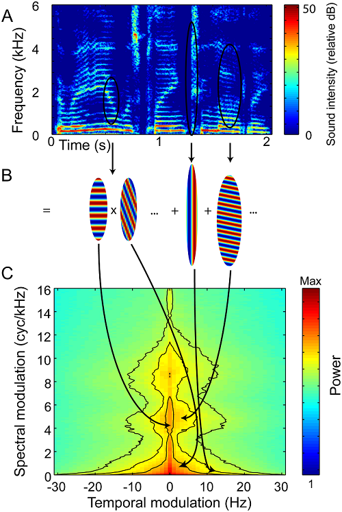
Figure 4.1
Modulation
spectra of spoken English. Spectrograms of spoken sentences (example sentence “The radio was
playing too loudly,” shown in A) are subjected to a two-dimensional Fourier
transform (2DFT) to calculate the sentence’s modulation spectrum (C). Just as
an ordinary Fourier transform represents a waveform as a superposition of sine
waves, a 2DFT represents a spectrogram as a superposition of “spectrotemporal ripples.” The spectrograms of the ripples
themselves look like zebra stripes (B). Their temporal modulation captures the
sound’s AM, and their spectral modulation captures spectral features such as
harmonics and formants.
Adapted from figure 1 of Elliott and Theunissen (2009) ) PLoS Comput Biol
5:e1000302.
But we cannot describe every
aspect of a spectrogram solely in terms of horizontal stripes that correspond
to particular the spectral modulations. There is also variation in time.
Particularly obvious examples are the short, sharp, broadband fricative and
plosive consonants which show up as vertical stripes in the spectrogram in figure
4.1A. In the modulation spectrum of a sound, these and
other “vertical” features are captured by “temporal modulations,” and this
occurs in a relatively intuitive manner. Temporal modulations simply measure
the amount of AM at some particular modulation rate, so high-frequency temporal
modulations capture fast changes in amplitude, low temporal modulation
frequencies capture slow changes in amplitude, and at 0 Hz temporal modulation
we find the sound’s grand average (constant) signal power.
Earlier, we mentioned that,
according to Greenberg (2006), speech sounds are characterized by syllabic energy
arcs, which are between 100 and 500 ms wide. These energy arcs should
correspond to temporal modulation frequencies between 10 and 2 Hz. The fact
that almost all the signal power in the speech modulation spectrum shown in figure
4.1C appears to be contained between +
and –10 Hz temporal modulation is therefore compatible with Greenberg’s
observations.
Hang on a minute. Did I just say a
temporal modulation of minus 10 Hz?
It is relatively easy to imagine what a temporal modulation of 10 Hz might
represent: Some property of the sound gets larger and then smaller and then
larger again ten times a second. But what, you may ask, is a temporal
modulation rate of minus 10 Hz
supposed to mean? You would be right to think that, in our universe, where time
never flows backward, a sound can hardly go thorough some cyclical changes once
every minus 0.1 s. Indeed, these “negative” temporal modulation frequencies
should simply be thought of as an expedient mathematical trick that allows us
to represent acoustic features in which frequency changes over time, and which
would show up as diagonal stripes in the spectrogram. The 2DFT captures such spectrotemporal modulations with diagonal ripples, and
these diagonals come in two flavors: They either rise, or they fall. In the
convention adopted here, a spectrotemporal ripple
with a negative temporal modulation corresponds to rising frequency
trajectories, while positive temporal frequencies correspond to falling
frequencies. The fact that the modulation spectrum shown in figure
4.1C is fairly symmetrical around 0 Hz
temporal modulation, thus, tells us that, in the sample of American English
sentences analyzed here, features with rising frequency content are just as
common as features with falling FM.
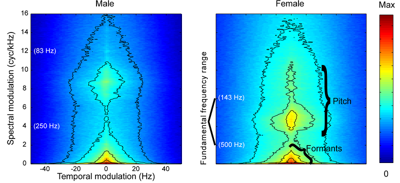
Figure 4.2
Modulation
spectra of male and female English speech.
From figure 2 of Elliott and
Theunissen (2009) PLoS Comput Biol 5:e1000302.
One very useful feature of the
modulation spectrum is that it separates out low spectral frequency, that is,
spectrally broad features such as the formants of speech, from high spectral
frequency features, such as harmonic fine structure associated with pitch. The
pitch of female speech tends to be noticeably higher than that of male speech,
but the formants of female speech differ less from those of male speech, which
presumably makes understanding speech, regardless of speaker gender,
substantially easier. This is readily apparent in the modulation spectra shown
in figure 4.2,
which are rather similar for the low spectral modulations (less than 3 cycles/kHz)
associated with the broad formant filters, but much more dissimilar for the
higher spectral modulations associated with pitch.
Given the crucial role of formants
in speech, we might therefore expect the meaning of the spoken sentence to be
carried mostly in the relatively low temporal and frequency modulations, and
one rather nice feature of Elliott and Theunissen’s
(2009) use of the modulation spectrum is that they were able to demonstrate
this directly. Modulation spectra, like ordinary Fourier transforms, are in
principle “invertible,” that is, you can use the spectrum to reconstruct the
original signal. Of course, if you blank out or modify parts of the modulation
spectrum before inversion, then you remove or modify the corresponding temporal
or spectral modulations from the original speech.
By testing comprehension of
sentences after filtering out various ranges of modulations, Elliott and Theunissen (2009) were able to demonstrate that spectral
modulations of less than 4 cycles/kHz and temporal modulations between 1 and 7
Hz are critical for speech intelligibility. They refer to this as the core region
of the human speech modulation spectrum, and it sits very much in those parts
of modulation space where we would expect the formants of speech to reside.
Filtering out modulations outside this core region has only a relatively small
effect on speech intelligibility, but may make it much harder to distinguish
male from female speakers, particularly if it affects spectral modulations
between 4 and 12 cycles/kHz, which, as we have seen in
figure 4.2,
encapsulate much of the differences in male versus female voice pitch. Examples
of such “modulation filtered” speech can be found in the online material accompanying
Elliott and Theunissen’s original (2009) paper, or on
the website accompanying this book. <flag>
Many artificial speech recognition
systems use a mathematical device that is conceptually closely related to the
modulation spectrum, known as the “dynamic cepstrum.”
Like the modulation spectrum, the cepstrum is
calculated as a Fourier transform along the frequency axis of the sound’s
spectrogram. The cepstrum can then be used to
separate out the low spectral modulations that are associated with the
relatively broadly tuned resonances of the vocal tract that mark the formants
of speech, and discard the high spectral modulations associated with pitch.
Pitch, thus, seems to add little
to speech comprehension, at least for English and most Indo-European languages.
(You can find examples of speech samples with altered pitch contours which
illustrate this on the book’s web site for <flag>). But it is worth
noting that many Asian languages are tonal, meaning that they may use pitch
trajectories to distinguish the meanings of different words. To give one
example: Translated into Mandarin Chinese, the sentence “mother curses the horse” becomes “ māma mà mă .” The symbols above the “a”s are
Pinyin1 tone markers, intended to indicate the
required pitch. Thus, the “ā” is
pronounced not unlike like the “a” in the English “bark,” but with a pitch much
higher than the speaker’s normal, neutral speaking voice. The “à,” in contrast, must be pronounced with
a rapidly falling pitch contour, and in the “ă”—particularly challenging for unaccustomed Western vocal
tracts—the pitch must first dip down low, and then rise again sharply, by well
over one octave, in a small fraction of a second. Remove these pitch cues, for
example, by filtering out spectral modulations above 7 cycles/kHz,
and the sentence becomes “mamamama,” which is gibberish in both Chinese and English.
One consequence of this use of pitch to carry semantic meaning in tonal
languages is that many current Western speech processing technologies, from
speech recognition software for personal computers to speech processors for
cochlear implants, are not well adapted to the needs of approximately one
quarter of the world’s population.
Nevertheless, even in tonal
languages, the lion’s share of the meaning of speech appears to be carried in
the formants, and in particular in how formant patterns change (how they are modulated)
over time. Relatively less meaning is encoded in pitch, but that does not mean
that pitch is unimportant. Even in Western, nontonal
languages, pitch may provide a valuable cue that helps separate a speech signal
out from background noise, or to distinguish one speaker from another. (We
shall return to the role of pitch as a cue in such auditory scene analysis
problems in chapter 6.) In chapter 3, we looked in detail at how pitch
information is thought to be represented in the auditory pathway, so let us now
look in more detail at how the auditory system distinguishes different classes
of speech sounds.
4.2 Categorical Perception of Speech Sounds
One crucial, but also
poorly understood, part of the neural processing of
speech is that sounds must be mapped onto categories. The physical properties
of a sound can vary smoothly continuously. Not only can we produce /a/ sounds
and /i/ sounds, but also all manner of vowels that
lie somewhere along the continuum between /a/ and /i/.
However, perceiving a sound as “between /a/ and /i/”
is unhelpful for the purpose of understanding speech. Our brains have to make categorical
decisions. A person who is talking to us may be telling us about his “bun” or
his “bin,” but it has to be one or the other. There is no continuum of objects
between “bun” and “bin.” Once we use speech sounds to distinguish different,
discrete objects, concepts, or grammatical constructs, we must subdivide the
continuous space of possible speech sounds into discrete categories. Such categorical
perception is therefore believed to be a key step in speech processing, and it
has attracted much interest among researchers. What are the criteria that our
brains use to distinguish sound categories? Are category boundaries arbitrary
parcellations of the set of all possible speech sounds, and do different
languages draw these boundaries differently? Or are there physical or
physiological laws that dictate where the boundaries should fall? And does the
human brain comprise specialized modules for recognizing such phoneme
categories that other animals lack, or is categorical
perception of speech sounds or vocalizations also seen in other animals?
Let us first consider the question
of phoneme boundaries. One thing that is readily apparent to most students of
foreign languages is that the phoneme boundaries are not the same in all languages.
German, for example, has its umlaut—“ä,” “ü,” and “ö”—effectively a set of
additional vowels that are lacking in English. Some Scandinavian languages have
even more vowels, such as the “å” and the “ø.” Thus, English lacks certain phoneme
categories that exist in other languages, but it also makes some distinctions other
languages do not. Japanese, for example, are famously unable to distinguish
between “r” and “l” sounds. This inability is not innate, however, but emerges
during the first year of life, as children are conditioned in their mother
tongue (Kuhl et al., 2006.). While these language-specific
differences suggest that phonetic boundaries are largely determined by the
environment we grow up in, they may nevertheless not be entirely arbitrary. In
a recent review, Diehl (2008) discussed two theories, the quantal
theory and the dispersion theory, which may help explain why phonetic category
boundaries are where they are. Both theories emerge from considerations of the
physical properties and limitations of the vocal tract.
To get a feeling for the ideas
behind quantal theory, let us start with a simple
experiment that you can try yourself. Make a long “ssssssss”
sound, and then, while keeping the sound going, move the tip of your tongue
very slowly backward in your mouth so as to gradually change the sound from /s/
to /sh/. When the tip of your tongue is near your
teeth, you will make an /s/, and with the tip of your
tongue further back against your palate you will make a /sh/.
So far so good, but you may notice that placing your tongue halfway between the
/s/ and /sh/ positions does not easily produce a
sound halfway between /s/ and /sh/. As you move your
tongue steadily forward or backward you may notice a very sudden transition (a “quantum
leap”) from /s/ to /sh/ or from /sh/
to /s/. Quantal theory posits that languages avoid
using speech sounds that are very close to such quantal
boundaries in the acoustics. We do not use speech sounds somewhere between /s/
and /sh/ because they would be too difficult to
pronounce reliably. Near a quantal boundary, a small
inaccuracy in the placement of the articulators will often lead to
disproportionately large changes in the sound produced, and therefore any
category of speech sounds that happened to live very close to a quantal boundary would be particularly easy to mispronounce
and mishear. Making sure that speech sound categories keep a respectful distance
from quantal boundaries would therefore make speech
more robust.
Dispersion theory (Liljencrants & Lindblom, 1972)
takes a different approach. It starts from the realization that there are
limits to the range of speech sounds a normal human vocal tract can produce.
The theory then makes the not unreasonable assumption that, to make speech
sound categories easily distinguishable, they should be widely spread out
(dispersed) across this space of all possible speech sounds. Figure
4.3 illustrates this for the case of vowel sounds. The
coordinate axes of figure 4.3
show the first and second formant frequency of a particular vowel. The
continuous contour shows the limits of the formant frequencies that a normal
human vocal tract can easily produce, while the dots show first and second
formant frequencies for some of the major vowel categories of the world’s
languages. It, indeed, looks as if the vowels are not positioned randomly
inside the space available within the contour, but instead are placed so as to
maximize their distances, which should help make them easily distinguishable.
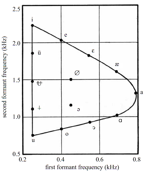
Figure 4.3
The contour shows the
pairings of possible F1/F2 formant frequencies, which are as distinct as they
could be, given the physical constraints of the human vocal tract. Symbols show
approximately where vowels of the world’s languages are located in this F1/F2
space.
Adapted from figure 7 of Diehl (2008)
Phil Trans Royal Soc B: Biological Sciences 363:965, with permission from the
Royal Society..
Thus, the quantal
and dispersion theories establish some ground rules for where phonetic category
boundary might fall, but there is nevertheless considerable scope for different
languages to draw up these boundaries differently, as we have seen. And this
means that at least some phoneme boundaries cannot be innate, but must be
learned, typically early in life. Interestingly, the learning of some of these
categorical boundaries appears to be subject to so-called critical or sensitive
developmental periods (Kuhl et al., 2008), so that
category distinctions that are learned in the early years of life are very hard
or impossible to unlearn in adulthood. Thus, Japanese speakers who have not
learned to differentiate between “r” and “l” early in life appear to find it
very difficult even to hear a difference between these sounds in adulthood. (We
will say more about sensitive periods in chapter 7.) However, that seems to be
an extreme case, and most learned phoneme boundaries do not bring with them an
inability to distinguish sounds that fall within a learned class. Thus, the
English language has no category boundary that distinguishes the vowels /ä/ or
/å/, yet adult native English speakers can learn very quickly to distinguish
and to recognize them.
So some phonetic category
boundaries, such as those between /r/ and /l/ or between /a/, /ä/, and /å/, are
therefore largely language specific and culturally determined, and children
pick them up in early infancy. But other phoneme boundaries seem fixed across many
languages, and may therefore be based on distinctions that are hard-wired into
the auditory system of all humans, or perhaps all mammals. For example, you may
recall that consonants differ either in their place or the manner of
articulation. Thus, /p/ and /t/ are distinguished by place of articulation (one
is made with the lips, the other with the tip of the tongue placed against the
top row of teeth), but /b/ and /p/ both have the same “labial” place of
articulation. What distinguishes /b/ from /p/ is that one is said to have a
“voiced” manner of articulation while the other is “unvoiced,” in other words
the /p/ in “pad” and the /b/ in “bad” differ mostly in their “voice onset time”
(VOT).2 In “pad,” there is a little gap of about 70
ms between the plosive /p/ sound and the onset of the vocal fold vibration that
mark the vowel /a/, while in “bad,” vocal fold vibration starts almost
immediately after the /b/, with a gap typically no greater than 20 ms or so.
Consequently, it is possible to morph a recording of the word “bad” to sound
like “pad” simply by lengthening the gap between the /b/ and the /a/. What is
curious about VOTs is that the length of VOTs does not seem to vary arbitrarily from one language to
the next. Instead, VOTs occur in no more than three distinct
classes, referred to as leading, short or long, which are conserved across the
world’s languages. In the leading category, voicing may start at about 100 ms
before the consonant, while short VOTs imply that
voicing starts 10 to 20 ms after the consonant, and long VOTs
mean that voicing starts about 70 ms after the consonant (Lisker
& Abramson, 1964). Leading voicing is not a typical feature of English, but
it is common in other languages such as Spanish, where, for example, “v” is
pronounced like a very soft /b/, so that the word “victoria” is pronounced “mbictoria.”
Several studies have shown that
animals, such as chinchillas (Kuhl & Miller 1978)
or quail (Kluender, Diehl, & Killeen, 1987), can be easily trained to discriminate stop consonants
with short or long VOTs. Thus the three VOT
categories may be “linguistic universals” because they are based on acoustic
distinctions that are particularly salient for the auditory systems not just of
humans but also of other animals.
4.3 Subcortical Representations of Speech Sounds and Vocalizations
You may recall from section
2.4, and in particular from figure 2.13, that the
inner ear and auditory nerve (AN) are thought to operate like a filter bank,
and firing rates along the tonotopic array of the
auditory nerve fiber bundle create a sort of “neurogram,”
a rate-place code for the acoustic energy distribution in the incoming sound.
The frequency resolution in that tonotopic rate-place
code is not terribly sharp, but it is easily sharp enough to capture formant
peaks. When we introduced the neurogram notion in figure
2.13, however, we did gloss over a small complication, which we now ought to
come clean about. We mentioned only in passing in section 2.4 that the majority
(roughly 80%) of AN fibers are high spontaneous rate
fibers that saturate—that is, they cannot fire any faster, once the sound at
their preferred frequency reaches a level of between 30 and 50 dB SPL. Over 30
years ago, Young and Sachs (1979) had already pointed out that this rate
saturation can have awkward consequences for the place-rate representation of
formants in the auditory nerve. Figure 4.4
illustrates some of their findings from a set of experiments in which they
recorded AN responses to artificial vowel sounds presented
at different sound levels.
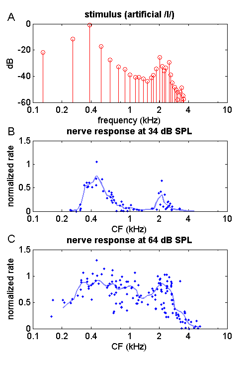
Figure 4.4
Responses
in the auditory nerve of the cat to a steady-state artificial vowel /I/. (A) power
spectrum of the vowel sound. It exhibits harmonics every 128 Hz, and formants
at approximately 0.4, 2, and 2.8 kHz. (B) Nerve fiber responses when the vowel
is presented at a relatively quiet 34 dB SPL. Each dot is the normalized evoked
firing rate of a single nerve fiber, plotted against each fiber’s CF. The
continuous line is a moving average along the frequency axis. The observed
nerve discharge rate distribution exhibits clear peaks near the stimulus
formant frequencies. (C) Nerve fiber responses when the sound is presented at a
moderately loud 64 dB SPL. Due to saturation of nerve fiber responses, the
peaks in the firing distributions are no longer clear. Based
on data published in Young and Sachs (1979).
Figure 4.4A shows the power spectrum of the
stimulus Sachs and Young used: an artificial vowel with harmonics every 128 Hz,
passed through a set of formant filters to impose formant peaks at about 400 Hz,
as well as at about 2,000 and 2,800 Hz. The resultant sound is not too different
from the human vowel /I/ (a bit like the “i” in
“blitz”). Note that the figure uses a logarithmic frequency axis, which
explains why the harmonics, spaced at regular 128-Hz intervals, appear to
become more densely packed at higher frequencies. Sachs and Young recorded
responses from many AN fibers in the anesthetized cat
to presentations of this sound at various sound levels. Figure
4.4B summarizes their
results for presentations of the artificial vowel at an
intensity of 34 dB SPL. Each point in figure
4.4B shows the response for a single nerve fiber.
The x-coordinate shows the nerve fiber’s characteristic frequency (CF), and the
y-coordinate shows the nerve fiber’s firing rate, averaged over repeated
presentations of the stimulus at 34 dB SPL, and normalized by subtracting the
nerve fiber’s spontaneous firing rate and dividing by the nerve fiber’s maximal
firing rate in response to loud pure tones at its CF. In other words, a normalized
rate of 0 means the neuron fires no more strongly than it would in complete
quiet, while a normalized rate of 1 means it fires almost as strongly as it
ever will. The gray continuous line in figure
4.4B shows a moving average across the observed
normalized firing rates for the AN fibers. This
averaged normalized firing rate as a function of CF appears to capture the
formant peaks in the stimulus quite nicely. So what’s the problem?
The problem is that 34 dB SPL is
really very quiet. Just the background hum generated by many air conditioning
systems or distant traffic noise will have higher sound levels. Most people
converse with speech sounds of an intensity closer to 65 to 70 dB SPL. But when
Sachs and Young repeated their experiment with the artificial vowel presented
at the more ”natural” sound level of 64 dB SPL, the firing rate distribution in
the auditory nerve was nothing like as pretty, as can be seen in figure 4.4C. The firing rate
distribution has become a lot flatter, and the formant peaks are no longer
readily apparent. The problem is not so much that the peaks in the firing rate
distribution at the formants have disappeared, but rather that the valley
between them has filled in. This is a classic example of the so-called dynamic
range problem. Most AN fibers saturate at relatively
modest sound intensities, and sounds don’t have to become very loud before the
AN fibers lose their ability to signal spectral contrasts like those between
the formant peaks and troughs in a vowel.
The curious thing, of course, is
that even though the representation of the formant peaks across the nerve fiber
array appears to become degraded as sound levels increase, speech sounds do not
become harder to understand with increasing loudness—if anything the opposite
is true. So what is going on?
There are a number of possible
solutions to the dynamic range problem. For example, you may recall from
chapter 2 that AN fibers come in two classes: High
spontaneous rate (HSR) fibers are very sensitive and therefore able to respond
to very quiet sounds, but they also saturate quickly; low spontaneous rate
(LSR) fibers are less sensitive, but they also saturate not nearly as easily.
The plots in figure 4.4
do not distinguish between these classes of AN fibers.
Perhaps the auditory pathway uses HSR fibers only for hearing in very quiet
environments. HSR fibers outnumber LSR fibers about four to one, so the large
majority of the nerve fibers sampled in figure
4.4 are likely to be HSR fibers, and using those to
encode a vowel at 64 dB might be a bit like trying to use night vision goggles
to see in bright daylight.
Young and Sachs (1979) also
proposed an alternative, perhaps better explanation when they noticed that,
even though the nerve fibers with CFs between 300 and
3,000 Hz shown in figure 4.3C may all fire at similarly high
discharge rates, they tend to phase lock to the formant frequencies close to
their own CF. For example, you might find a 500-Hz fiber that is firing
vigorously, but at an underlying 400-Hz rhythm. In that case you might conclude
that the dominant frequency component in that frequency range is the frequency
signaled by the temporal firing pattern (400 Hz) even if this is not the nerve
fiber’s preferred frequency (500 Hz). Such considerations led Young and Sachs
(1979) to propose a response measure that takes both firing rate and phase
locking into account. This response measure, the “average localized synchronized
rate” (ALSR), quantifies the rate of spikes that are locked to the CF of the
neuron. In the previous example, the ALSR would be rather low for the 500-Hz
neuron, since most spikes are synchronized to the 400-Hz formant. The ALSR
measure of auditory nerve discharges reflects formant frequencies much more
stably than ordinary nonsynchronized rate-place codes
could.
Whether your auditory brainstem
solves the dynamic range problem by computing the ALSR, by listening
selectively either to HSR or to LSR fibers depending on sound level, or by
relying on some other as yet unidentified mechanism is not known. However, we
can be pretty certain that your auditory brainstem does solve this problem, not
only because your ability to understand speech tends to be robust over wide
sound level ranges, but also because electrophysiological recordings have shown
that so-called chopper neurons in the ventral cochlear nucleus can represent
formants in a much more sound level invariant manner than the auditory nerve
fibers do (Blackburn & Sachs, 1990).
At the level of the auditory
brainstem, as well is in the major midbrain nuclei such as the inferior colliculus or the medial geniculate,
and to some extent even in primary auditory cortex, this representation is
thought to retain a somewhat spectrographic character. The pattern of neural
discharges mostly reflects the waxing and waning of acoustic energy in the
particular frequency bands to which these neurons happen to be tuned. But much
experimental evidence suggests that this representation is not very isomorphic,
in the sense that neural firing patterns in the brainstem and midbrain do not
simply and directly reflect the rhythms of speech. Nor do the temporal response
properties of neurons in the midbrain or cortex appear to be tuned to match the
temporal properties of speech particularly well. Evidence for this comes from
studies like those by Miller and colleagues (2002), who have analyzed response
properties of midbrain and cortex neurons using synthetic dynamic ripple
stimuli and reverse correlation. The dynamic ripple sounds they used are
synthetic random chords that vary constantly and randomly in their frequency and
amplitude. The rationale behind these experiments rests on the assumption that,
at some periods, just by chance, this ever changing stimulus will contain
features that excite a particular neuron, while at other times it will not. So,
if one presents a sufficiently long random stimulus, and then asks what all
those stimulus episodes that caused a particular neuron to fire had in common,
one can characterize the neuron’s response preferences. Often this is done by a
(more or less) simple averaging of the spectrogram of the stimulus episodes
that preceded a spike, and the resulting spike-triggered average of the
stimulus serves as an estimate of the neuron’s spectrotemporal
receptive field (STRF).
You may recall from our
discussions in chapter 2 that auditory neurons can be modeled, to a coarse
approximation, as linear filters. For example, in figure 2.12, we illustrated
similarities between auditory nerve fibers and so-called gamma-tone filters.
Now, in principle, we can also try to approximate auditory neurons in the
central nervous system with linear filter models (only the approximation risks
becoming ever cruder and more approximate as each level of neural processing
may contribute nonlinearities to the neural response properties). The way to
think of a neuron’s STRF is as a sort of spectrographic display of the linear
filter that would best approximate the neuron’s response properties.
Consequently, we would expect a neuron to fire vigorously only if there is a
good match between the features of the STRF and the spectrogram of the
presented sound.
Figure 4.5A shows such an example of an STRF
estimated for one neuron recorded in the auditory midbrain of the cat. The STRF
shows that this particular neuron is excited by sound at about 9 kHz and the
excitation kicks in with a latency of about 10 ms.
There are inhibitory frequency regions both above and below the neuron’s
preferred frequency. But we also see that the excitatory region near 9 kHz is followed
by “rebound inhibition,” which should shut off this neuron’s firing after about
30 ms of response. The STRF would thus predict that continuous, steady-state
sounds are not particularly effective stimuli for this neuron.
In section 4.1, we discussed the
dynamic properties of speech, and saw how its characteristic amplitude and
frequency modulations can be captured by its modulation spectrum. We also saw how
the modulation spectrum is generated from the sound’s spectrogram by two-dimensional
Fourier transformation. Now, if the STRF of a neuron is a sort of
spectrographic display of the spectral and temporal features that a neuron
prefers, we ought to be able to apply a similar thought process here, and
transform the neuron’s STRF with a 2DFT to reveal what sort of spectral and
temporal modulations the neuron might respond to with particular vigor. To use
the technical term, we can use the 2DFT of the STRF to obtain the neuron’s “modulation
transfer function” (MTF). Figure 4.5B
shows the MTF obtained in this manner from the STRF shown in figure 4.5A.
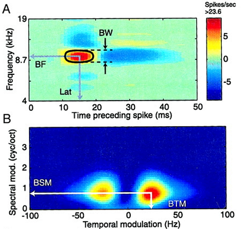
Figure 4.5
(A) Spectrotemporal receptive field of a neuron recorded in the
auditory thalamus of the cat. BW: spectral band width, BF: best frequency, Lat:
response latency. (B) Modulation transfer function for the same neurons. BSM, best
spectral modulation, BTM, best temporal modulation.
Reproduced from figure 1 of Miller et
al. (2002), with permission from the American Physiological Society..
When many neurons are
characterized in this manner, it is possible to investigate what range of
temporal and spectral modulations the population of neurons, on average, might
be able to represent effectively through equivalent modulations of their own
firing rates. We can then ask, is this population MTF well
matched to the modulations encountered in speech? Figure
4.6 shows population MTFs
determined in this manner for the main auditory thalamic relay station to the
cortex, the ventral part of the medial geniculate (MGv), and for the primary auditor cortex of the cat.
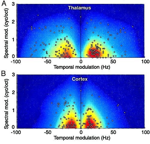
Figure 4.6
(A) Population MTF of
the auditory thalamus (MGv) cat. The dots show best
temporal and spectral modulation values for individual neurons. The gray values
show the averaged MTF. (B) Population MTF for cat A1.
Reproduced from figure
8 of Miller et al. (2002), with permission from the American Physiological
Society.
Comparing the population MTFs of auditory thalamus and cortex shown in figure 4.6 to the speech modulation
spectra shown in figures 4.1C and 4.2,
we notice that the neural MTFs at these, still
relatively early, auditory processing stations are not obviously well matched
to the temporal modulations characteristic of speech. However, it would
probably have been surprising if they were. For starters, the MTFs shown in figure
4.6 were recorded in cats, and the cat midbrain is
hardly likely to be optimized for the processing of human speech. However, we
have no reason to assume that the population MTFs of
human thalamus or primary auditory cortex would look much different. The shape
of the population MTF can provide some insights into the nature of the neural
code for sounds in the midbrain that are likely to be true for most mammals.
The best temporal modulation frequencies for these neurons are often higher
than they would need to be for the purposes of speech encoding (extending out
to 50 Hz and above while speech modulations rarely exceed 30 Hz). In contrast,
the best frequency modulations are not nearly high enough to capture the pitch
part of the speech modulation spectrum, but they do appear quite well matched
to the frequency modulation spectra of formants. We saw in chapters 2 and 3
that, already at the level of the auditory nerve, frequency tuning of individual
nerve fibers is not usually sharp enough to resolve the harmonics that would
reveal the pitch of a periodic sound, and the low-pass nature of the population
MTF suggests that midbrain neurons cannot resolve harmonics in the sound’s
spectrum either.
Another striking mismatch between
the speech modulation spectrum and the neural population MTF can be seen at
temporal modulation frequencies near zero. Speech modulation spectra have a lot
of energy near 0-Hz temporal modulation, which reflects the fact that, on
average, there is some sound almost all the time during speech. However, as one
ascends the auditory pathway toward cortex, auditory neurons appear
increasingly unwilling to respond to sustained sound with sustained firing.
Instead, they prefer to mark sound onsets and offsets with transient bursts of
firing, and then fall silent. Slow temporal modulations of their firing rates
are consequently rare. With this emphasis on change in the spectrum, rather
than sustained sound energy levels, the representation of sounds in the
midbrain and above resembles the derivative of the spectrogram with respect to
time, but since speech sounds are rarely sustained for long periods of time,
this emphasis on time-varying features does not change the representation
dramatically. In fact, as we shall see later, even at the level of the primary
visual cortex, speech sounds appear to be represented in a manner that is
perhaps more spectrographic (or neurographic) than
one might expect. Consequently, much interesting processing of speech remains
to be done when the sounds arrive at higher-order cortical fields. Where and
how this processing is thought to take place will occupy us for much of the
rest of this chapter.
4.4 Cortical Areas Involved in Speech Processing: An Overview
Before we start our
discussion of the cortical processing of speech sounds in earnest, let us
quickly revise some of the key anatomical terms, so we know which bit is which.
Figure 4.7 shows anatomical drawings of the human
cerebral cortex. Figure 4.7A
shows the left side of the cortex, reminding you that the cortex on each
hemisphere is subdivided into four lobes: The occipital lobe at the back deals
mostly with visual processing; the parietal lobe deals with touch, but also
integrates information across sensory modalities to keep track of the body’s
position relative to objects and events around us; the frontal lobe is involved
in planning and coordinating movements, short-term working memory, and other cognitive
functions; and, finally, the temporal lobe is involved in hearing, but also in
high-level vision, general object recognition, and the formation of long-term
memories.
In the human brain, many of the
auditory structures of the temporal lobe are not visible on the surface, but
are tucked away into the sylvian fissure, which forms
the boundary between the temporal, frontal and parietal lobes. Figure
4.7B
therefore shows a view of the human brain from above, with the left frontal and
parietal lobes cut away to show the upper bank of the temporal lobe. Most of
the auditory afferents from the thalamus terminate in Heschl’s
gyrus, where primary auditory cortex is found in
humans. To the front and back of Heschl’s gyrus lie the planum polare and the planum temporale, where second-order auditory belt areas are
situated.
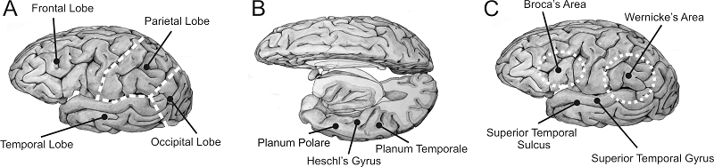
Figure 4.7
(A) Drawing of a
lateral view of the human brain, showing the four principal lobes. (B) Human
cortex seen from above, with the frontal and parietal lobe cut away to expose
the superior bank of the temporal lobe, where the primary auditory cortex (Heschl’s gyrus) and auditory belt
areas (planum temporale and
polare) are situated. (C) Lateral view showing higher-order
cortical areas commonly associated with higher-order auditory processing and
speech.
Original artwork kindly provided by
Jo Emmons (www.joemmons.com).
But the processing of speech
certainly also involves cortical areas well beyond the auditory areas on the
upper bank of the temporal lobe. A few of the other key areas are shown in figure 4.7C,
including the superior temporal gyrus (STG) and sulcus (STS), and Broca’s and Wernicke’s areas. The latter two are both named after nineteenth-century
neurologists who associated damage to these areas with disturbances of either
speech production (Broca’s aphasia) or speech
comprehension (Wernicke’s aphasia. See the book’s
website for short video clips showing patients with Broca’s
and Wernicke’s aphasia.) Note that the definitions of
Broca’s and Wernicke’s
areas are not based on anatomical landmarks, but instead derived from case
studies of patients with injuries to these parts of the brain. Since the damage
caused by such injuries is rarely confined to precisely circumscribed regions, the
exact boundaries of Broca’s and Wernicke’s
areas are somewhat uncertain, although a consensus seems to be emerging among neuroanatomists that Broca’s area
should be considered equivalent to the cytoarchitectonically
defined and well-circumscribed Brodmann areas 44 and
45. In any case, both Wernicke’s and Broca’s areas clearly lie either largely or entirely
outside the temporal lobe, which is traditionally associated with auditory
processing. Note also that, while both hemispheres of the cortex have frontal,
parietal, occipital, and temporal lobes, as well as Heschl’s
gyri and superior temporal sulci,
much clinical evidence points to the left hemisphere playing a special role in
speech processing, and Broca’s and Wernicke’s areas appear normally to be confined largely or
wholly to the left hemisphere.
4.5 The Role of Auditory Cortex: Insights from Clinical Observations
Paul Broca, who lived from 1824 to 1880, and in whose honor one
of the brain areas we just encountered is named, was one of the first to
observe that speech processing may be asymmetrically distributed in cortex. He
stated that the left hemisphere was “dominant” for language. Broca chose his words carefully. The left hemisphere’s
dominance is not meant to imply that the right hemisphere contributes nothing
to speech comprehension or production. Rather, the left hemisphere, in most but
not all individuals, is capable of carrying out certain key speech processing
functions even if the right hemisphere is not available to help, but the right
hemisphere on its own would not succeed. We might envisage the situation as similar
to that of a lumberjack who, if forced to work with one hand only, would be
able to wield his axe with his right hand, but not with his left. This “righthand-dominant lumberjack” would nevertheless work at
his best if allowed to use both hands to guide his axe, and his left hand would
normally be neither idle nor useless.
Since Broca’s
time, a wealth of additional clinical and brain imaging evidence has much
refined our knowledge of the functional roles of the two brain hemispheres and
their various areas in both the production and the comprehension of speech.
Much of that work was nicely summarized in a review by Dana Boatman (2004),
from which we present some of the highlights.
Much of the research into human
speech areas has been driven forward by clinical necessity, but perhaps
surprisingly not as much from the need to understand and diagnose speech
processing deficits as from the desire to cure otherwise intractable epilepsy
by surgical means. In these epilepsy surgeries, neurosurgeons must try to
identify the “epileptic focus,” a hopefully small piece of diseased brain
tissue that causes seizures by triggering waves of uncontrollable hyperexcitation which spread through much of the patient’s
brain. Successful identification and removal of the epileptic focus can cure
the patient of a debilitating disease, but there are risks. For example, if the
operation were to remove or damage one of the brain’s crucial speech modules, the
patient would be left dumb or unable to understand speech. That would be a
crippling side effect of the operation one would like to avoid at all cost. So,
the more we know about the location of such crucial brain regions, the better the
surgeon’s chances are to keep the scalpel well away from them.
One complicating factor which neurosurgeons
have appreciated for a long time is that the layout of cortex is not absolutely
identical from one person to the next, and it is therefore desirable to test each
individual patient. One such test that has been administered frequently since
the 1960s is the so-called Wada procedure (Wada & Rasmussen, 1960), during
which a short-acting anesthetic (usually sodium amytal)
is injected into the carotid artery, one of the main blood supply routes for
the cerebral hemispheres of the brain. After injecting the anesthetic on either
the left or right side only, one can then try to have a conversation with a
patient who is literally half asleep, because one of his brain hemispheres is
wide awake, while the other is deeply anesthetized. Records of such Wada tests
have revealed that approximately 90% of all right-handed patients and about 75%
of all left-handed patients display Broca’s classic
“left hemisphere dominance” for speech. The remaining patients are either
“mixed dominant” (i.e., they need both hemispheres to process speech) or have a
“bilateral speech representation” (i.e., either hemisphere can support speech
without necessarily requiring the other). Right hemisphere dominance is
comparatively rare, and seen in no more than 1 to 2% of the population.
The Wada procedure has its
usefulness—for example, if we needed to perform surgery on the right brain
hemisphere, it would be reassuring to know that the patient can speak and
comprehend speech with the spared left hemisphere alone. However, often one
would like more detailed information about the precise localization of certain
functions than the Wada test can provide. To obtain more detailed information,
neurosurgeons sometimes carry out electrocortical
mapping studies on their patients. Such mappings require preparing a large part
of one of the patient’s brain hemispheres for focal electrical stimulation
either by removing a large section of the skull to make the brain accessible
for handheld electrodes, or by implanting a large electrode array over one of
the hemispheres. During the actual mapping, the patient receives only local
anesthetic and analgesics, and is therefore awake and can engage in
conversation or follow simple instructions.
The patients are then tested on
simple speech tasks of varying level of complexity. The simplest, so called acoustic-phonetic
tasks, require only very simple auditory discriminations; for example, the
patient is asked whether two syllables presented in fairly quick succession are
the same or different. The next level, so called phonological tasks, require a slightly deeper level of analysis of the
presented speech sounds. For example, the patient might be asked whether two
words rhyme, or whether they start with the same phoneme. Note that neither acoustic-phonetic nor phonological tasks requires
that the tested speech sounds be understood. For example, I can easily repeat
the syllable “shmorf,” I can tell that it rhymes with
“torf,” and that “shmorf”
and “torf” do not start with the same phoneme. I can
do all this even though both “shmorf” and “torf” are completely meaningless to me. The ability to use
speech sounds for meaningful exchanges requires a further so-called lexical-semantic
level of analysis, which typically involves asking a patient to carry out
simple instructions (such as “please wiggle the ring finger on your left hand”)
or to answer questions of varying level of grammatical complexity.
While the patients are grappling
with these acoustic, phonological, or semantic tasks, the surgeon will sneakily
send small bursts of electric current to a particular spot on their brain. This
current is just large enough to disrupt the normal activity of the neurons in
the immediate vicinity of the stimulating electrodes, and the purpose of this
is to test whether this highly localized disruption makes any obvious
difference to the patient’s ability to perform the task.
In such electrocortical
mapping studies, one does observe a fair degree of variation from one patient
to another, as no two brains are exactly alike. But one can nevertheless observe
clear trends, and Dana Boatman (2004) has summarized which parts of cortex
appear to be essential for acoustic, phonological, or semantic tasks across a
large numbers of patients. The results of her analysis are shown in figure 4.8.
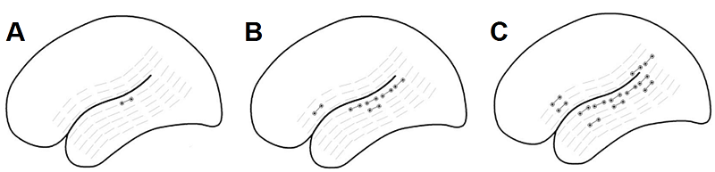
Figure 4.8
Sites
where acoustic (A), phonological (B), or lexical-semantic (C) deficits can be
induced by disruptive electrical stimulation. The light gray symbols show locations on perisylvian cortex that were tested by applying disruptive
electrical stimulation. The black symbols show sites where such stimulation
interfered with the patient’s ability to perform the respective task.
Reproduced from figures 1 through 3
of Boatman (2004),. Cognition 92:47-65., with
Copyright (2004) permission from Elsevier.
The data in figure 4.8 suggest a hierarchical
arrangement. The more complex the task, the larger the number
of cortical sites that seem to make a critical contribution because disruptive
stimulation at these sites impairs performance. Acoustic-phonetic tasks
(figure 4.8A)
are not easily disrupted. Only at a single spot on the superior temporal sulcus (STS) could electrical stimulation reliably
interfere with phonetic processing in all patients. Phonological processing (figure 4.8B) requires a greater
degree of analysis of the speech sounds, and it seems to involve large parts of
STS, as well as some points on Broca’s area on the
frontal lobe, since focal stimulation of any of these areas impairs
performance. Lexical-semantic tasks (figure
4.8C) are yet more complex, and seem to involve yet
more cortical territory because they are even more vulnerable to disruption.
Focal stimulation not just of the superior temporal gyrus
(STG), STS, and Broca’s area, but also of Wernicke’s area in the parietal lobe can disrupt the performance
of this type of tasks.
In figure
4.8 we also notice that the sites where one can
disrupt processing on the next higher level of complexity always appear to
include the sites that were involved in the lower processing levels. That is
perhaps unsurprising. If some focal electrical stimulation perturbs my
perception of speech sounds to the point where I can no longer tell whether two
words spoken in sequence were the same or different, then it would be odd if I
could nevertheless tell whether those word rhymed, or what they meant. XXX
The clinical data thus suggests a
cortical processing hierarchy, which begins with acoustic-phonetic processing
in or near primary auditory cortex, and engages ever-increasing amounts of
cortical territory as the brain subjects vocalizations
to phonological and semantic analysis. But the clinical data cannot provide
much detail on what exactly each particular cortical area contributes to the
process. For example, the fact that semantic processing of sounds can be
disrupted by electrical stimulation of parts of Wernicke’s
area does not mean that important steps toward this semantic processing may not
have already begun at much earlier levels in the cortical hierarchy. In fact,
some results from animal research might be interpreted as evidence for
“semantic preprocessing” from the earliest levels.
4.6 The Representation of Speech and Vocalizations in Primary Auditory Cortex
Since semantic
processing involves finding the “meaning” of a particular speech sound or
animal vocalization, one can try to investigate semantic processing by
comparing neural responses to “meaningful” sounds with responses to sounds that
are “meaningless” but otherwise very similar. One simple trick to make speech
sounds incomprehensible, and hence meaningless, is to play them backward. Time
reversing a sound does not change its overall frequency content. It will flip
its modulation spectrum along the time axis, but since speech modulation
spectra are fairly symmetrical around t
= 0 (see figure 4.1C), this does not seem to matter much. Indeed, if you have
ever heard time-reversed speech, you may know that it sounds distinctly speechlike, not unlike someone talking in a foreign
language (You can find examples of such time reversed speech in the book’s
website <flag>). Of
course, one can also time reverse the vocalizations of other animals, and
indeed, in certain songbird species, brain areas have been identified in which
neurons respond vigorously to normal conspecific songs, but not to
time-reversed songs (Doupe and Konishi,
1991). Typically, the songbird brain areas showing such sensitivity to time
reversal seem to play an important role in relating auditory input to motor
output, for example, when a bird learns to sing or monitors its own song.
Interestingly, Xiaoqin
Wang and colleagues (1995) have used the same trick in marmosets, a species of
new world monkey, and found that already in primary auditory cortex, many
neurons respond much more vigorously to natural marmoset twitter calls than to
time-reversed copies of the same call. Could it be that marmoset A1 neurons
fire more vigorously to the natural calls because they are “meaningful,” while
the time-reversed ones are not? If the same natural and time-reversed marmoset
calls are presented to cats, one observes no preferential responses in their A1
for the natural marmoset calls (Wang & Kadia,
2001), perhaps because neither the natural nor the reversed marmoset calls are
particularly meaningful for cats.
However, the interpretation of
these intriguing data is problematic. One complicating factor, for example, is
the fact that the relationship between the number of spikes fired by some
neuron during some relatively long time interval and the amount of information
or meaning that can be extracted from the neuron’s firing pattern is not
straightforward. A more vigorous response does not necessarily convey
proportionally more information. This was clearly illustrated in a study by Schnupp and colleagues (2006), who used the same marmoset
calls as those used by Wang et al. (1995), but this time played them either to
naïve ferrets, or to ferrets who had been trained to recognize marmoset twitter
calls as an acoustic signal that helped them find drinking water. For the
trained ferrets, the marmoset calls had thus presumably become “meaningful,”
while for the naïve ferrets they were not. However, neither in the naïve nor
the trained ferrets did primary auditory cortex neurons respond more strongly
to the natural marmoset calls than to the time-reversed ones. Instead, these
neurons responded vigorously to either stimuli, but many of these neurons
exhibited characteristic temporal firing patterns, which differed
systematically for different stimuli. These temporal discharge patterns were
highly informative about the stimuli, and could be used to distinguish
individual calls, or to tell normal from time-reversed ones. However, these
neural discharge patterns had to be “read out” at a temporal resolution of 20
ms or finer; otherwise this information was lost. Figure
4.9 illustrates this. Schnupp
and colleagues (2006) also showed that training ferrets to recognize these
marmoset vocalizations did not change the nature of this temporal pattern code,
but did make it more reliable and hence more informative.
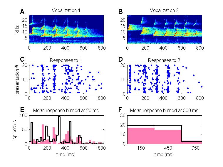
Figure 4.9
(A, B) Spectrograms of
two marmoset “twitter calls.” (C, D) Dot rasters showing responses of a neuron in ferret
primary auditory cortex to these sounds. Each dot represents one nerve impulse,
each row of dots an impulse train fired in response to a single presentation of
the corresponding stimulus. The neuron fires similar mean spike counts but with
different temporal discharge patterns in response to each stimulus. (E, F)
Responses shown in C and D are plotted as histograms, showing the mean firing
rate poststimulus onset, with the responses to
stimulus 1 shown in gray, those to stimulus 2 in black. At fine temporal
resolutions (small histogram bin width, e.g., 20 ms shown in E) the differences
in the response patterns are very clear and, as shown by Schnupp
et al. (2006), contain much information about stimulus identity. However, at
coarser temporal resolutions (300 ms bin width, shown in F), the responses look
very similar, and information about stimulus identity is lost.
These results indicate that the
representation of complex stimuli like vocalization or speech at early stages
of the cortical processing hierarchy is still very much organized around
“acoustic features” of the stimulus, and while this feature-based
representation does not directly mirror the temporal fine structure of the
sound with submillisecond precision, it does
nevertheless reflect the time course of the stimulus at coarser time
resolutions of approximately 10 to 20 ms. It may or may not be a coincidence
that the average phoneme rate in human speech is also approximately one every
20 ms, and that, if speech is cut into 20-ms-wide strips, and each strip is
time-reversed and their order is maintained, speech remains completely
comprehensible (Saberi & Perrott,
1999) (A sound example demonstrating this can be found on the book’s website.
<flag>).
Further evidence for such a
feature-based representation of vocalizations and speech sounds in mammalian A1
comes from a recent study by Engineer and colleagues (2008), who trained rats
to recognize consonants of American English. The rats were trained to
distinguish nonsense syllables that differed only in their onset consonant:
“pad” from “bad,” “zad” from “shad,” “mad” from “nad,” and so on. Some of these distinctions the rats
learned very easily, while they found others more difficult. Engineer and
colleagues then proceeded to record responses to these same syllables from
hundreds of neurons in the auditory cortex of these animals. These responses
are reproduced here in figure 4.10 as neurogram-dot raster displays. Each panel shows the
responses of a large number of primary auditory cortex neurons, arranged by
each neuron’s best frequency along the y-axis. The x-axis shows time after stimulus
onset. The panels zoom in on the first 40 ms only to show the response to the
onset consonant.
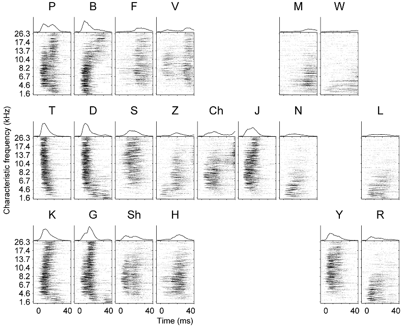
Figure 4.10
Responses
or rat A1 neurons to 20 different consonants.
Adapted by permission from Macmillan Publishers, Ltd: Nature
Neuroscience: Figs 1 and 2 of Engineer et al. (2008) Nat Neurosci
11:603-608., copyright (2008)
Figure 4.10 shows that the A1 neurons
normally respond to the onset syllable with one or occasionally with two bursts
of activity, but the bursts do not all start at the same time, nor are they all
equally strong. Instead, they vary systematically, depending on the sound
stimulus and the neuron’s frequency tuning. In fact, the firing pattern is
still very much like the neurogram responses we saw
in figure 2.13 for auditory nerve fiber
responses. When presented with an /m/ or an /n/, which
contain little acoustic energy at high frequencies, the high-frequency A1 neurons
fail to fire. Conversely, in response to an /s/, which
contains little energy at low frequencies, only the high-frequency neurons
respond. This interplay between frequency sensitivity and the acoustic
properties of the stimulus leads to each vowel having its own response pattern
in across the population of cortical neurons. Interestingly, when Engineer and
colleagues (2008) used pattern classifier algorithms similar to those used by Schnupp et al. (2006) to quantify the differences between
the cortical activity patterns evoked by the different vowels, they noticed
that these differences predicted how easily a rat would learn to distinguish
the sounds. Thus, /m/ and /n/ evoked rather similar response patterns, and rats
found it very hard to distinguish them, but /p/ and /b/ evoked rather different
response patterns, and rats learned to distinguish the sounds easily.
The responses to /p/ and /b/ shown
in figure 4.9
are, in fact, particularly interesting, because they exhibit a phenomenon that had
previously been described by Steinschneider, Fishman,
and Arezzo (2003) in the primary auditory cortex of rhesus monkeys and by Eggermont (1995) in cortex of cats. In response to /p/, the
low- to mid-frequency neurons produce two bursts of impulses, while in response
to /b/ they produce just one. In fact, the second burst of action potentials in
the response to /p/ is not strictly a response to /p/, but a response to the
onset of voicing, to the /a/ in the syllables “pad” and “bad” that were
presented to the animals. There is, of course, an /a/ in
“bad” as well, yet the response to it is suppressed in the low- and mid-frequency
neurons, probably due to a phenomenon of “forward masking.” You may recall from
section 4.2 that the key distinguishing feature between /p/ and /b/ is that the
former has a longer VOT; that is, in “pad” the gap between the consonant and
the vowel may be some 60 to 70 ms long, while in “bad” it may be no longer than
20 ms. The longer gap in “pad” gives the neurons time to recover from forward
masking and to respond vigorously to both the /p/ and the /a/, whereas in
“bad,” forward masking much reduces the response to the /a/. Neural response
patterns tend to transition fairly abruptly from single-peaked to double-peaked
responses when a “ba” sound is morphed to a “pa” by
lengthening the VOT. Forward masking is thus one aspect of neural processing that
leads to a deviation in the neural firing patterns from what might be expected
on the basis of a purely spectrographic representation, and it may be the
responsible for the categorical perceptual boundaries associated with VOTs that we discussed in section 4.2. Thus, although
responses at the earliest cortical processing levels appear to represent purely
acoustic-phonetic aspects of vocalizations, their response properties may
nevertheless account for at least some aspects of categorical perception.
4.7 Processing of Speech and Vocalizations in Higher-Order Cortical Fields
As we have just seen,
the representation of animal vocalizations or speech sounds in early stages of
auditory cortex still appears to be fairly “raw”, and rather directly related
to physical stimulus attributes. A somewhat categorical distinction between /p/
and /b/ based on a relative suppression of a response to the voice onset seems
to be as good as it gets. One might reasonably assume that neural responses would
become fairly specific if they reflected the result of lexical-semantic
processing, yet most studies indicate that neurons in early cortical processing
stages are not very selective but respond more or less vigorously to all manner
of vocalizations as well as to other sounds from inanimate objects. It
therefore looks as if many of the most interesting aspects of speech and
vocalization processing apparently occur “beyond” the primary auditory fields.
Unfortunately, when it comes to
the study of speech and vocalization processing in higher-order cortical areas,
obtaining the very detailed data against which to test particular theories is very
difficult. One of the main experimental approaches for this type of work is noninvasive
functional imaging in normal human volunteers, using techniques like positron
emission tomography (PET) or functional magnetic resonance imaging (fMRI). These approaches can yield some interesting results.
For example, a study by Scott and colleagues (2000) provided intriguing
evidence that parts of the left anterior STG may be activated selectively by
intelligible speech. This conclusion was based on a comparison of cortical
activation patterns obtained either with normal speech sounds or with speech rendered
unintelligible by inverting sound along the frequency axis (You can find an
example of such spectrally rotated speech on the book’s website <flag>).
However, as Scott herself points
out in a comprehensive review (Scott & Wise, 2004), word deafness (i.e.,
the inability to recognize the meaning of words) only rarely results from
damage to the left STG alone, and usually occurs only in patients who suffered
injury to the STG on both sides. This highlights one methodological problem
inherent in functional brain imaging studies. When a particular area of the
brain appears to “light up” under the scanner, what we really see is a
marginally greater blood supply to this area during some particular stimulus
regime than during another. As a measure of brain activity, this is very
indirect. One problem is that it reveals only the tip of the iceberg; it shows
which brain area blushed significantly more under the effort of the neural
processing it carried out than some neighboring area. And here “significantly more” is to be understood
in the statistical sense, meaning that the difference can be measured with a
fair degree of confidence, not that it is very large. Neighboring areas may
have made crucial contributions to the processing, but these fail to show up in
the functional scan because they were performed “relatively effortlessly.”
Another limitation of fMRI and PET stems from their inherently poor temporal
resolution, as they effectively measure responses of the brain’s vasculature that
reflect the relatively slowly changing metabolic demands of the neural tissue.
Consequently, fMRI and PET cannot resolve any brain processes
that occur on timescales faster than a few seconds. As we saw in the previous
section, deciphering the cortical code is likely to require a temporal
resolution approximately 1,000-fold faster. Consequently, a number of elegant
theories that have recently emerged remain largely untestable
with functional imaging techniques. For example, it has been suggested that
certain brain areas may be specialized for processing slow aspects of speech,
such as “prosody”—that is, the overall melody and rhythm of a speech, which
conveys emotional undertones or labels sentences as questions or statements—while
other brain areas may specialize in processing fast features, such as formant
transitions that identify individual speech sounds (Poeppel
& Hickok, 2004). Whether, or to what extent, this is really true we will know
only when techniques that provide more direct observations of neural activity
on a millisecond timescale become widely available.
Detailed and direct observations
are, of course, possible in animal experiments, where microelectrodes can be
implanted directly in the areas of interest. However, the layout of high-order
cortical fields may not be identical from one species of mammal to the next,
and humans not only have a uniquely rich, complex vocal communication system,
they also have substantially larger cortices than almost any other mammal. Studies
carried out on some of our primate cousins, such as rhesus macaques, may
nevertheless provide interesting insights that are likely to be representative
of the processes we would expect to take place in human brains.
Based on anatomical observations,
it has been suggested that auditory cortical areas in primate brain may be
organized into two more or less discrete processing streams (Romanski et al., 1999): a dorsal stream, which may be
concerned mostly with identifying sound source locations, and a ventral stream,
which is thought to play the lead role in identifying sounds. Anatomical
evidence from tracer studies indicates that this ventral stream should run from
primary auditory cortex via medial belt (secondary) areas to anterior STG and
inferotemporal cortex, and from there finally to areas
in the ventral prefrontal cortex (vPFC). Recognizing
and distinguishing different types of vocalizations or spoken words should most
certainly be a “ventral stream task,” and the notion that the ventral stream
may form the “sound-meaning interface” in human speech processing is often
discussed in the literature (Hickok & Poeppel,
2004; Scott & Wise, 2004).
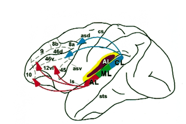
Figure 4.11
Putative
dorsal and ventral processing streams in macaque auditory cortex, as suggested
from anatomical tracer studies.
Adapted by permission from the author and from Macmillan Publishers Ltd: Figure 3D of Romanski et al. (1999). Nat Neurosci 2:1131-1136, copyright (1999).
Against this background, a recent
set of experiments by Russ and colleagues (2008) is therefore of particular
interest, as these investigators were able to record activity from individual
neurons in the STG and the vPFC of awake rhesus
macaques, who were listening to ten very different types of rhesus vocalization
calls. These calls are acoustically very distinct, the animals make different
calls in different social situations, and there is little doubt that each of
these calls therefore has a different meaning for the animals. If neurons in
the ventral stream indeed represent the meaning of a vocalization, then one
might expect these neurons to be rather selective in their response to these
calls; that is, each neuron might respond to only a small subset of calls with
similar meanings. We might also expect that this specificity would increase as
one ascends along the ventral path from STG to vPFC.
Finally, we would not expect neurons in the vPFC to
be very interested in minute acoustic details, such as the temporal fine
structure of the sound, nor to represent much information in the temporal fine
structure of its discharges. After all, if I pronounce a particular word the
meaning of my utterance does not depend on whether I speak fast or slowly or
introduce small gaps between the syllables, and even speaking very rapidly I
would find it difficult to convey more than two or three concepts per second on
average. Meaning therefore unfolds relatively slowly, and the temporal fine
structure of sounds becomes irrelevant once their meaning has been identified.
Consequently, if neurons in vPFC, at the end of the
ventral stream, really represent the abstracted, lexical meaning of a
vocalization rather than the sound itself, we would not expect their temporal
firing patterns to convey much stimulus-related information on a millisecond
timescale.
What makes the experiments by Russ
and colleagues (2008) so interesting and surprising is that they produced a
wealth of data that clearly runs counter to all these expectations. Neurons in
the STG and vPFC are not very selective in their
responses. The large majority of neurons respond vigorously (with >50% of
their maximal firing rate) to more than half of the vocalizations tested. Nor
do responses become more specific as one ascends from STG to vPFC—if anything, the reverse is true. But both STG and vPFC neurons convey a great deal of information about which
of the vocalizations was presented in the temporal fine structure of their
discharges. Using spike pattern classification techniques identical to those
used by Schnupp and colleagues (2006) to analyze
neural discharge patterns recorded in ferret A1, Russ et al. (2008) were able
to show that responses of neurons in macaque STG and vPFC
also need to be decoded at a resolution of a few milliseconds if the individual
vocalizations are to be correctly identified. Furthermore, the reliance on
precise temporal patterning of the discharges is, if anything, larger in vPFC than in STG.
Do the results of Russ and
colleagues (2008) mean that our intuitions about how our brain “ought to”
represent the meaning of sounds are simply wrong, and that the meaning of a
sound is never represented explicitly through invariant, sparse, and
categorical responses? Perhaps, but alternatively it could be that, to see such
meaning-specific responses, one needs to look outside the auditory pathway.
After all, meaning is abstracted somewhat beyond the level of any particular
sensory modality, and it is not uncommon that the same meaning can be conveyed with
both sounds and pictures. Interestingly, recent work by Quian
Quiroga and colleagues (2009) found neurons in
structures buried inside the temporal lobe, such as the hippocampus, the amygdala, and the entorhinal
cortex, that may respond to pictures of some specific familiar object, say a
landmark or a person or a pet, and these same neurons may also respond to that object’s
name, either spoken or written. These object-specific neurons are highly
selective for stimulus category, responding typically to only one or two
stimulus objects out of over a hundred tested. At the same time, they are
unselective in the sensory modality, as they frequently respond as vigorously
to a spoken name or a characteristic sound as to a visual image. They have long
response latencies (300 ms or so for images, 500 ms or more for sounds), and
their discharges appear not to reflect acoustic features of the auditory
waveform in any way.
It is curious that such “semantic”
responses to the meaning of sound have been observed only in structures such as
the amygdala (which is thought to process the
emotional significance of stimuli, e.g., “are they scary or not”) or the
hippocampus (which seems to serve as the gateway to long-term episodic memory).
As we have seen, even at the highest levels of the auditory “what stream,”
neural responses appear overwhelmingly tuned to acoustic stimulus properties,
not their semantics. Perhaps we simply haven’t yet looked hard enough for semantically
tuned responses in higher-order auditory cortex. It is worth bearing in mind,
however, that such semantic responses may also be rare in the hippocampus, the amygdala, and entorhinal cortex. Quian Quiroga and colleagues
(2009) tested 750 neurons, and found that fewer than 4% of neurons (25 in total) seemed to be object specific and responsive to sound.
If semantically tuned neurons formed a small subset of the neural population in
higher-order auditory cortex, and if their responses were very highly selective
and “sparse,” then they could have slipped through the net in previous
investigations.
4.8 Visual Influences
The brain does, of
course, rely mostly on acoustic information to process speech and
vocalizations, but it will also happily incorporate visual information if this
is useful. Listeners who suffer from hearing impairments or who have to operate
under difficult conditions with large amounts of background noise often find it
much easier to understand a speaker if they can also observe the movement of
his or her mouth, and “lip read.” At a very basic level, lip reading can be
helpful simply because of the temporal cueing it provides: Sounds you hear when
the speaker’s mouth is not moving are bound to be purely background noise. But
since the lips (together with the tongue and the soft palate) are one of the
chief articulators used to shape speech sound, visual observation of the lips
provides information that can help distinguish different phonemes and influence
their perception.
This is vividly illustrated by a
visual-auditory illusion known as the McGurk effect (McGurk & MacDonald, 1976). To create the McGurk effect, a video is made showing a person
articulating the syllables “gaga” over and over again. The video is then
synchronized with a soundtrack of the person speaking the syllables “baba.” If you watch a McGurk
video, your ears will hear the syllables “baba,” but
you can also see that the lips are not closed at the onset of the syllables, so
your eyes tell you that the syllables you heard could not have started with a
labial plosive. You will therefore not perceive the /ba/
that was actually delivered to your ears, but instead hear a /da/ or a /tha/, as these are
acoustically similar to the actual sound, but are articulated by the tip of the
tongue, which is not visible, so the eyes do not provide evidence against them.
The /da/ or /tha/ you
perceive is, in effect, the most plausible compromise between the /ga/ that is shown and the /ba/
that is played. You can find a McGurk effect video on
the book’s web site <flag>. Try watching it, and then just listening to
it with your eyes closed. The difference in the sound you hear depending on
whether your eyes are open or not is quite compelling.
With your eyes closed you will clearly hear that the movie’s sound track
consists entirely of the syllables “baba,” but when
you open your eyes the sound appears to change instantly to “dada” or “thatha”.
The McGurk
effect nicely illustrates how visual information can directly and powerfully
influence and enrich our auditory perception of speech sounds, and it probably
exercises this influence through visual inputs that feed directly into the
auditory cortex. A number of electrophysiological studies have reported
responses in auditory cortex to visual stimuli (Bizley
et al., 2007; Brosch, Selezneva,
& Scheich, 2005). Also, imaging experiments have
shown that auditory cortex can be activated by silent lip reading (Calvert et
al., 1997), and activity in auditory cortex can be enhanced when speech is
presented along with a movie showing the face of a speaker (Callan
et al.,2003). Selective enhancement of responses to
vocalization stimuli that are seen as well as heard has also been described in
monkeys (Ghazanfar et al., 2005).
Thus, visual information can contribute
significantly to the neural processing of vocalization stimuli, but it is
important to remember that the role of the visual modality is nevertheless a
minor one. Telecommunications technology has advanced to the point where video
telephony is becoming widely available, yet most of us do not feel the need for
it. Nobody would think it a practical idea to rely on the video only and switch
the sound off. Educational policies that discourage profoundly deaf children
from learning sign language and instead try to teach them to understand normal
speech through lip reading alone are well intended, but nevertheless badly
flawed. They ignore the important fact that the most of the articulatory
gestures we use to encode our thoughts in speech, such as voicing and all the
subtle movements of the tongue and the soft palate, simply cannot be observed
by looking at a speaker’s face. They are accessible to us only through their
acoustic fingerprints, which a healthy auditory system can decipher with
surprising ease.
4.9 Summary
As we have seen,
speech most likely evolved from initially rather simple vocal communication
systems, comprising perhaps less than a dozen or so distinct messages, such as
mating calls, alarm calls, pup calls, threats, and a few others. From these
humble beginnings, speech evolved into a staggeringly sophisticated
communication system, in which humans can combine and recombine a relatively
modest number of speech sounds to communicate a seemingly limitless variety of
ideas. These ideas reach the ear of the listener encoded as a more or less
continuous stream of amplitude- and frequency-modulated sound. But not all
spectral and temporal modulations in the speech signal are equally important.
Relatively coarse levels of detail (temporal modulations between 1 and 7 Hz and
spectral modulations of less than 4 cycles/kHz) are
usually sufficient for a successful decoding of the message.
The auditory system is thought to
decipher speech sounds through a hierarchy of successive analyses, which operate
on different timescales. Acoustic-phonetic analysis examines amplitude and
frequency modulations in the incoming sound in order to detect and characterize
speech sounds within the signal, phonological processing aims to reconstruct
how speech sounds are arranged to form syllables and words, while lexical-semantic
analysis aims to decipher the meaning of the sounds. Most of these processing
steps are thought to involve areas of cortex, particularly those on the upper
part of the temporal lobe, but also some frontal and parietal areas,
particularly in the left cerebral hemisphere, but many important details of how
these cortical areas operate remain obscure.