3 Periodicity and Pitch Perception
Physics, Psychophysics, and Neural Mechanisms
- 3.1 Periodicity Is the Major Cue for Pitch
- 3.2 The Relationship between Periodicity, Frequency Content, and Pitch
- 3.3 The Psychophysics of Pitch Perception
- 3.4 Pitch and Scales in Western Music
- 3.5 Pitch Perception by Nonhuman Listeners
- 3.6 Algorithms for Pitch Estimation
- 3.7 Periodicity Encoding in Subcortical Auditory Pathways
- 3.8 Periodicity Coding in Auditory Cortex
- 3.9 Recapitulation: The Paradoxes of Pitch Perception
The American National Standards Institute (ANSI, 1994) defines pitch as “that auditory attribute of sound according to which sounds can be ordered on a scale from low to high.” Thus, pitch makes it possible for us to appreciate melodies in music. By simultaneously playing several sounds with different pitches, one can create harmony. Pitch is also a major cue used to distinguish between male and female voices, or adult and child voices: As a rule, larger creatures have lower pitch (see chapter 1). And pitch can help convey meaning in speech—just think about the rising melody of a question (“You really went there?”) versus the falling melody of a statement (“You really went there!”); or you may be aware that, in tonal languages like Mandarin Chinese, pitch contours differentiate between alternative meanings of the same word. Finally, pitch also plays less obvious roles, in allowing the auditory system to distinguish between inanimate sounds (most of which would not have pitch) and animal-made sounds (many of which do have a pitch), or to segregate speech of multiple persons in a cocktail party. Pitch therefore clearly matters, and it matters because the high pitch of a child’s voice is a quintessential part of our auditory experience, much like an orange-yellow color would be an essential part of our visual experience of, say, a sunflower.
The ANSI definition of pitch is somewhat vague, as it says little about what properties the “scale” is meant to have, nor about who or what is supposed to do the ordering. There is a clear consensus among hearing researchers that the “low” and “high” in the ANSI definition is to be understood in terms of musical notes, and that the ordering is to be done by a “listener.” Thus, pitch is a percept that is evoked by sounds, rather than a physical property of sounds. However, giving such a central role to our experience of sound, rather than to the sound itself, does produce a number of complications. The most important complication is that the relationship between the physical properties of a sound and the percepts it generates is not always straightforward, and that seems particularly true for pitch. For example, many different sounds have the same pitch—you can play the same melody with a (computer-generated) violin or with a horn or with a clarinet (Sound Example "Melodies and Timbre" on the book’s Web site <flag>). What do the many very different sounds we perceive as having the same pitch have in common?
As we tackle these questions, we must become comfortable with the idea that pitch is to be judged by the listener, and the correct way to measure the pitch of a sound is, quite literally, to ask a number of people, “Does this sound high or low to you?,” and hope that one gets a consistent answer. A complete understanding of the phenomenon of pitch would need to contain an account of how the brain generates subjective experiences. That is a very tall order, indeed, and as we shall see, even though the scientific understanding of pitch has taken great strides in recent decades, a large explanatory gap still remains.
But we are getting ahead of ourselves. Even though pitch is ultimately a subjective percept rather than a physical property of sounds, we nevertheless know a great deal about what sort of sounds are likely to evoke particular types of pitch percept. We shall therefore start by describing the physical attributes of sound that seem most important in evoking particular pitches, briefly review psychoacoustics of pitch perception in people and animals, and briefly outline the conventions used for classifying pitches in Western music, before moving on to a discussion of how pitch cues are encoded and processed in the ascending auditory pathway.
3.1 Periodicity Is the Major Cue for Pitch
Probably the most important determinant of the pitch of a sound is its “periodicity.” A sound is periodic when it is composed of consecutive repetitions of a single short segment (figure 3.1). The duration of the repeated segment is called the period (abbreviated T). In figure 3.1, the period is 1 s. Sometimes, the whole repeated segment is called the period—we shall use both meanings interchangeably. Only a small number of repetitions of a period are required to generate the perception of pitch (Sound Example "How many repetitions are required to produce pitch?" on the book’s Web site). Long periods result in sounds that evoke low pitch, while short periods result in sounds that evoke high pitch.
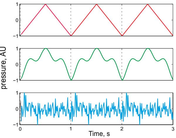
Figure 3.1
Three examples of periodic sounds with a period of 1 s. Each of the three examples consists of a waveform that repeats itself exactly every second.
Periodicity is, however, most often quantified not by the period, but rather by the “fundamental frequency” (F0 in Hertz), which is the number of times the period repeats in 1 s (F0=1/T). For example, if the period is 1 ms (1/1,000 s), the fundamental frequency is 1,000 Hz. Long periods correspond to low fundamental frequencies, usually evoking low pitch, while short periods correspond to high fundamental frequencies, usually evoking high pitch. As we will see later, there are a number of important deviations from this rule. However, for the moment we describe the picture in its broad outlines, and we will get to the exceptions later.
This is a good point to correct a misconception that is widespread in neurobiology texts. When describing sounds, the word “frequency” is often used to describe two rather different notions. The first is frequency as a property of pure tones, or a property of Fourier components of a complex sound, as we discussed in chapter 1, section 1.3. When we talk about frequency analysis in the cochlea, we use this notion of frequency, and one sound can have many such frequency components at once. In fact, we discussed the frequency content of complex sounds at length in chapter 1, and from now on, when we use the terms “frequency content” or “frequency composition,” we will always be referring to frequency in the sense of Fourier analysis as described in chapter 1. However, we introduced here another notion of frequency, which is the fundamental frequency of a periodic sound and the concomitant pitch that sound evokes.
Although for pure tones the two notions of frequency coincide, it is important to realize that these notions of frequency generally mean very different things: Pitch is not related in a simple way to frequency content as we defined it in chapter 1. Many sounds with the same pitch may have very different frequency composition, while sounds with fairly similar frequency composition may evoke different pitches. In particular, there is no “place code” for pitch in the cochlea—the place code of the cochlea is for frequency content, not for pitch. In fact, sounds with the same pitch may excite different positions along the cochlea, while sounds with different pitch may excite identical locations along the cochlea. In order to generate the percept of pitch, we need to process heavily the signals from the cochlea and often to integrate information over many cochlear places. We will learn about some of these processes later. For the rest of this chapter, we will use F0 to signify fundamental frequency.
As a rule, periodic sounds are said to evoke the perception of pitch at their F0. But what does that mean? By convention, we use the pitch evoked by pure tones as a yardstick with respect to which we judge the pitch evoked by other sounds. In practical terms, this is performed by matching experiments: A periodic sound whose pitch we want to measure is presented alternately with a pure tone. Listeners are asked to change the frequency of the pure tone until it evokes the same pitch as the periodic sound. The frequency of the matching pure tone then serves as a quantitative measure of the pitch of the tested periodic sound. In such experiments, subjects most often set the pure tone so that its period is equal to the period of the test sound ( Sound Example "Pitch Matching" on the book’s Web site;).
At this point, it is time to mention complications that have to be added on top of the rather simple picture presented thus far. As we will see again and again, every statement about the relationships between a physical characteristic of sounds and the associated perceptual quality will have many cautionary notes attached (often in “fine print”). Here are already a number of such fine print statements:
First, periodic sounds composed of periods that are too long do not evoke pitch at their F0. They may instead be perceived as a flutter—a sequence of rapidly repeating discrete events—or they may give rise to a sensation of pitch at a value that is different from their period (we will encounter an example later in this chapter). To evoke pitch at the fundamental frequency, periods must be shorter than about 25 ms (corresponding to an F0 above about 40 Hz). Similarly, if the periods are too short, less than about 0.25 ms (i.e., the F0 is higher than 4,000 Hz), the perception of pitch seems to deteriorate (Sound Example "The Range of Periods that Evoke Pitch" on the book’s Web site). For example, the ability to distinguish between different F0 values declines substantially, and intervals do not sound quite the same.
Second, as alluded to earlier, many sounds that are not strictly periodic also have pitch. If the periods are absolutely identical, the sound might be called strictly periodic, but it is usually enough for subsequent periods to be similar to each other for the sound to evoke pitch. We will therefore not think of periodicity as an all-or-none property. Rather, sounds may be more or less periodic according to the degree to which successive periods are similar to each other. We will consider later ways of measuring the amount of periodicity, and relate it to the saliency or strength of the evoked pitch. Sounds that are not strictly periodic but do evoke pitch are typical—human voices are rarely strictly periodic (figure 3.2 and Sound Example "Vowels are not strictly periodic" on the book's Web site)—and the degree of periodicity that is sufficient for evoking pitch can be surprisingly small, as we will see later. Pitch can even be evoked by presenting a different sound to each ear, each of which, when presented alone, sounds completely random; in those cases, it is the interaction between the sounds in the two ears that creates an internal representation of periodicity that is perceived as pitch.

Figure 3.2
Four periods of the vowel /a/ from natural speech. The periods are similar but not identical (note the change in the shape of the feature marked by the arrows between successive periods).
3.2 The Relationship between Periodicity, Frequency Content, and Pitch
In chapter 1, we discussed Fourier analysis—the expression of any sound as a sum of sine waves with varying frequencies, amplitudes, and phases. In the previous section, we discussed pure tones (another name for pure sine waves) as a yardstick for judging the pitch of a general periodic sound. These are two distinct uses of pure tones. What is the relationship between the two?
To consider this, let us first look at strictly periodic sounds. As we discussed in chapter 1, there is a simple rule governing the frequency representation of such sounds: All their frequency components should be multiples of F0. Thus, a sound whose period, T, is 10 ms (or 0.01 s, corresponding to a F0 of 100 Hz as F0 = 1/T) can contain frequency components at 100 Hz, 200 Hz, 300 Hz, and so on, but cannot contain a frequency component at 1,034 Hz. Multiples of F0 are called harmonics (thus, 100 Hz, 200 Hz, 300 Hz, and so on are harmonics of 100 Hz). The multiplier is called the number, or order, of the harmonic. Thus, 200 Hz is the second harmonic of 100 Hz, 300 Hz is the third harmonic of 100 Hz, and the harmonic number of 1,000 Hz (as a harmonic of 100 Hz) is ten.
It follows that a complex sound is the sum of many pure tones, each of which, if played by itself, evokes a different pitch. Nevertheless, most complex sounds would evoke a single pitch, which may not be related simply to the pitch of the individual frequency components. A simple relationship would be, for example, for the pitch evoked by a periodic sound to be the average of the pitch that would be evoked by its individual frequency components. But this is often not the case: For a sound with a period of 10 ms, that evokes a pitch of 100 Hz, only one possible component, at 100 Hz, has the right pitch. All the other components, by themselves, would evoke the perception of other, higher, pitch values. Nevertheless, when pure tones at 100 Hz, 200 Hz, and so on are added together, the overall perception is that of a pitch at F0, that is, of 100 Hz.
Next, a periodic sound need not contain all harmonics. For example, a sound composed of 100, 200, 400, and 500 Hz would evoke a pitch of 100 Hz, in spite of the missing third harmonic. On the other hand, not every subset of the harmonics of 100 Hz would result in a sound whose pitch is 100 Hz. For example, playing the “harmonic” at 300 Hz on its own would evoke a pitch at 300 Hz, not at 100 Hz. Also, playing the even harmonics at 200, 400, 600 Hz, and so on, together, would result in a sound whose pitch is 200 Hz, not 100 Hz. This is because 200 Hz, 400 Hz, and 600 Hz, although all harmonics of 100 Hz (divisible by 100), are also harmonics of 200 Hz (divisible by 200). It turns out that, in such cases, it is the largest common divisor of the set of harmonic frequencies that is perceived as the pitch of the sound. In other words, to get a sound whose period is 10 ms, the frequencies of the harmonics composing the sound must all be divisible by 100 Hz, but not divisible by any larger number (equivalently, the periods of the harmonics must all divide 10 ms, but must not divide any smaller number).
Thus, for example, tones at 200 Hz, 300 Hz, and 400 Hz, when played together, create a sound with a pitch of 100 Hz. The fact that you get a pitch of 100 Hz with sounds that do not contain a frequency component at 100 Hz was considered surprising, and such sounds have a name: sounds with a missing fundamental. Such sounds, however, are not uncommon. For example, many small loudspeakers (such as the cheap loudspeakers often used with computers) cannot reproduce frequency components below a few hundred Hertz. Thus, deep male voices, reproduced by such loudspeakers, will “miss their fundamental.” As long as we consider pitch as the perceptual correlate of periodicity, there is nothing strange in pitch perception with a missing fundamental.
But this rule is not foolproof. For example, adding the harmonics 2,100, 2,200, and 2,300 would produce a sound whose pitch would be determined by most listeners to be about 2,200 Hz, rather than 100 Hz, even though these three harmonics of 100 Hz have 100 as their greatest common divisor, so that their sum is periodic with a period of 10 ms (100 Hz). Thus, a sound composed of a small number of high-order harmonics will not necessarily evoke a pitch percept at the fundamental frequency (Sound Example "Pitch of 3-Component Harmonic Complexes" on the book's Web site ;).
There are quite a few such exceptions, and they have been studied in great detail by psychoacousticians. Generally, they are summarized by stating the periodicity as the determinant of pitch has existence regions: combinations of periodicity and harmonic numbers that would give rise to a perception of pitch at the fundamental frequency. The existence regions of pitch are complex, and their full description will not be attempted here (see Plack & Oxenham, 2005).
What happens outside the existence regions? As you may have noticed if you had a chance to listen to Sound Example "Pitch of 3-Component Harmonic Complexes" on the book’s Web site, such a sound does not evoke pitch at its F0, but it does evoke a pitch, which is, in this case, related to its frequency content: This sound would cause the cochlea to vibrate maximally at the location corresponding to 2,100 Hz. There are a number of other sound families like this one, where pitch is determined by the cochlear place that is maximally stimulated. Pitch is notably determined by the cochlear place in cochlear implant users, whose pitch perception is discussed in chapter 8. Some authors would call this type of pitch “place pitch” and differentiate it from the periodicity pitch we discuss here. The important fact is that the extent of the existence regions for periodicity pitch is large, and consequently, for essentially all naturally occurring periodic sounds, the period is the major determinant of pitch.
We already mentioned that there are sounds that are not strictly periodic but are sufficiently periodic to evoke a pitch. What about their frequency composition? These sounds will usually have a frequency content that resembles a series of harmonics. Figure 3.3 (Sound Example "Non-Periodic Sounds That Evoke Pitch" on the book's Web site) shows three stimuli with this characteristic. The first is a strictly periodic sound to which white noise is added. The frequency content of this sound is the sum of the harmonic series of the periodic sound and the white noise. Thus, although it is not a pure harmonic series, such a spectrum is considered to be a minor variation on a harmonic series.
The second example comes from a family of stimuli called iterated repeated noise (also called iterated ripple noise, or IRN), which will play an important role later in the chapter. To create such a sound, we take a segment of white noise, and then add to it a delayed repeat of the same noise (i.e., an identical copy of the noise that has been shifted in time by exactly one period). Any leftovers at the beginning and the end of the segment that have had no delayed copies added to them are discarded. This operation can be repeated (iterated) a number of times, hence the name of this family of stimuli. The sound in figure 3.3B was created using eight iteration steps. In the resulting sound, successive sound segments whose duration is equal to the delay are not identical, but nevertheless share some similarity to each other. We will therefore call them “periods,” although strictly speaking they are not. The similarity between periods decreases with increasing separation between them, and disappears for periods that are separated by more than eight times the delay. As illustrated in figure 3.3B, the spectrum of this sound has peaks at the harmonic frequencies. These peaks have a width—the sound contains frequency components away from the exact harmonic frequencies—but the similarity with a harmonic spectrum is clear.
The third example is a so-called AABB noise. This sound is generated by starting with a segment of white noise whose length is the required period. This segment is then repeated once. Then a new white noise segment with the same length is generated and repeated once. A third white noise segment is generated and repeated once, and so on. This stimulus, again, has a partial similarity between successive periods, but the partial similarity in this case consists of alternating episodes of perfect similarity followed by no similarity at all. The spectrum, again, has peaks at the harmonic frequencies, although the peaks are a little wider (figure 3.3C).
These examples suggest that the auditory system is highly sensitive to the similarity between successive periods. It is ready to suffer a fair amount of deterioration in this similarity and still produce the sensation of pitch. This tolerance to perturbations in the periodicity may be related to the sensory ecology of pitch—periodic sounds are mostly produced by animals, but such sounds would rarely be strictly periodic. Thus, a system that requires precise periodicity would be unable to detect the approximate periodicity of natural sounds.
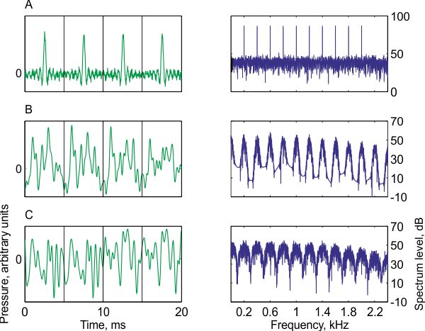
Figure 3.3
Three examples of nonperiodic sounds that evoke a strong pitch perception. Each sound is displayed as a time waveform (left) showing four quasi-periods (separated by the gray lines), and the corresponding long-term power spectrum (right) showing the approximate harmonic structure. All sounds have a pitch of 200 Hz. (A) A harmonic complex containing harmonics 1 to 10 of 200 Hz with white noise. The white noise causes the small fluctuations between the prominent peaks to be slightly different from period to period. (B) Iterated repeated noise with eight iterations [IRN(8)]. The features of the periods vary slowly, so that peaks and valleys change a bit from one period to the next. (C) AABB noise. Here the first and second period are identical, and again the third and fourth periods, but the two pairs are different from each other.
3.3 The Psychophysics of Pitch Perception
Possibly the most important property of pitch is its extreme stability, within its existence region, to variations in other sound properties. Thus, pitch is essentially independent of sound level—the same periodic sound, played at different levels, evokes the same (or very similar) pitch. Pitch is also independent of the spatial location of the sound. Finally, the pitch of a periodic sound is, to a large extent, independent of the relative levels of the harmonics composing it. As a result, different musical instruments, playing sounds with the same periodicity, evoke the same pitch (as illustrated by Sound Example "Melodies and Timbre" on the book's Web site ). Once we have equalized loudness, spatial location, and pitch, we call the perceptual quality that still differentiates between sounds timbre. Timbre is related (among other physical cues) to the relative levels of the harmonics. Thus, pitch is (almost) independent of timbre.
Since pitch is used to order sounds along a single continuum, we can try to cut this continuum into steps of equal size. There are, in fact, a number of notions of distance along the pitch continuum. The most important is the notion of distance used in music. Consider the distance between 100 Hz and 200 Hz along the pitch scale. What would be the pitch of a sound at the corresponding distance above 500 Hz? A naïve guess would be that 600 Hz is as distant from 500 Hz as 200 Hz is from 100 Hz. This is, however, wrong. Melodic distances between pitches are related not to the frequency difference but rather to the frequency ratio between them. Thus, the frequency ratio of 100 and 200 Hz is 200/100 = 2. Therefore, the sound at the same distance from 500 Hz has a pitch of 1,000 Hz (1,000/500 = 2). Distances along the pitch scale are called intervals, so that the interval between 100 and 200 Hz and the interval between 500 and 1,000 Hz are the same. The interval in both cases is called an octave—an octave corresponds to a doubling of the F0 of the lower-pitched sound. We will often express intervals as a percentage (There is a slight ambiguity here: When stating an interval as percentage, the percentage is always relative to the lower F0.): The sound with an F0 that is 20% above 1,000 Hz would have F0 of 1,200 [= 1,000*(1+20/100)] Hz, and the F0 that is 6% above 2,000 Hz would be 2,120 [= 2,000*(1+6/100)] Hz. Thus, an octave is an interval of 100%, whereas half an octave is an interval of about 41% [this is the interval called “tritone” in classical music, for example, the interval between B and F]. Indeed, moving twice with an interval of 41% would correspond to multiplying the lower F0 by (1 + 41/100)*(1 + 41/100) » 2. On the other hand, twice the interval of 50% would multiply the lower F0 by (1 + 50/100)*(1 + 50/100) = 2.25, an interval of 125%, substantially more than an octave.
How well do we perceive pitch? This question has two types of answers. The first is whether we can identify the pitch of a sound when presented in isolation. The capability to do so is called absolute pitch or perfect pitch (the second name, while still in use, is really a misnomer—there is nothing “perfect” about this ability). Absolute pitch is an ability that is more developed in some people than in others. Its presence depends on a large number of factors: It might have some genetic basis, but it can be developed in children by training, and indeed it exists more often in speakers of tonal languages such as Chinese than in English speakers.
The other type of answer to the question of how well we perceive pitch has to do with our ability to differentiate between two different pitches presented sequentially, an ability that is required in order to tune musical instruments well, for example. The story is very different when sounds with two different pitches are presented simultaneously, and we will not deal with it here. For many years, psychoacousticians have studied the limits of this ability. To do so, they measured the smallest “just noticeable differences” (JNDs) that can be detected by highly trained subjects. Typical experiments use sounds that have the same timbre (e.g., pure tones, or sounds that are combinations of the second, third, and fourth harmonics of a fundamental). One pitch value serves as a reference. The subject hears three tones: The first is always the reference, and the second and third contain another presentation of the reference and another sound with a slightly different pitch in random order. The subject has to indicate which sound (the second or third) is the odd one out. If the subject is consistently correct, the pitch difference between the two sounds is decreased. If the subject makes an error, the pitch difference is increased. The smaller the pitch difference between the two sounds, the more likely it is for the subject to make an error. Generally, there won't be a sharp transition from perfect to chance-level discrimination. Instead, there will be a range of pitch differences in which the subject mostly answers correctly, but makes some mistakes. By following an appropriate schedule of decreases and increases in the pitch of the comparison sound, one can estimate a “threshold” (e.g., the pitch interval that would result in 71% correct responses). Experienced subjects, under optimal conditions, can perceive at threshold the difference between two sounds with an interval of 0.2% (e.g., 1,000 and 1,002 Hz) (Dallos, 1996). This is remarkably small—for comparison, the smallest interval of Western music, the semitone, corresponds to about 6% (e.g., 1,000 and 1,060 Hz), about thirty times larger than the JND of well-trained subjects.
However, naïve subjects generally perform much worse than that. It is not uncommon, in general populations, to find a subject who cannot determine whether two sounds are different even for intervals of 10 or 30% (Ahissar et al., 2006; Vongpaisal & Pichora-Fuller, 2007). The performance in such tasks also depends on some seemingly unimportant factors: For example, discrimination thresholds are higher (worse) if the two sounds compared are shifted in frequency from one trial to the next, keeping the interval fixed (the technical term for such a manipulation is “roving”), than if the reference frequency is fixed across trials (Ahissar et al., 2006). Finally, the performance can be improved dramatically with training. The improvement in the performance of tasks such as pitch discrimination with training is called “perceptual learning,” and we will say a bit more about it in chapter 7.
In day-to-day life, very accurate pitch discrimination is not critical for most people (musicians are a notable exception). But this does not mean that we cannot rely on pitch to help us perceive the world. Pitch is important for sound segregation—when multiple sounds are simultaneously present, periodic sounds stand out over a background of aperiodic background noise. Similarly, two voices speaking simultaneously with different pitches can be more easily segregated than voices with the same pitch. The role of pitch (and periodicity) in grouping and segregating sounds will be discussed in greater detail in chapter 6.
3.4 Pitch and Scales in Western Music
As an application for the ideas developed in the previous sections, we provide here a brief introduction to the scales and intervals of Western music. We start by describing the notions that govern the selection of pitch values and intervals in Western music (in other words, why are the strings in a piano tuned the way they are). We then explain how this system, which is highly formalized and may seem rather arbitrary, developed.
We have already mentioned the octave—the interval that corresponds to doubling F0. Modern Western music is based on a subdivision of the octave into twelve equal intervals, called the semitones, which correspond to a frequency ratio of 21/12 » 1.06 (in our terminology, this is an interval of about 6%). The “notes,” that is, the pitches, of this so-called chromatic scale are illustrated in figure 3.4. Notes that differ by exactly one octave are in some sense equivalent (they are said to have the same chroma), and they have the same name. Notes are therefore names of “pitch classes” (i.e., a collection of pitches sharing the same chroma), rather than names of just one particular pitch. The whole system is locked to a fixed reference: the pitch of the so-called middle A, which corresponds to an F0 of 440 Hz. Thus, for example, the note “A” denotes the pitch class that includes the pitches 55 Hz (often the lowest note on the piano keyboard), 110 Hz, 220 Hz, 440 Hz, 880 Hz, 1,760 Hz, and so on.
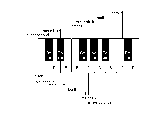
Figure 3.4
The chromatic scale and the intervals of Western music. This is a schematic representation of part of the keyboard of a piano. The keyboard has a repeating pattern of twelve keys, here represented by a segment starting at a C and ending at a D one octave higher. There are seven white keys and five black keys lying between neighboring white keys except for the pairs E and F, and B and C. The interval between nearby keys (white and the nearest black key, or two white keys when there is no intermediate black key) is a semitone. The names of the intervals are given with respect to the lower C. Thus, for example, the interval between C and F# is a tritone, that between the lower and upper Cs is an octave, and so on.
The names of the notes that denote these pitch classes are complicated (figure 3.4). For historical reasons, there are seven primary names: C, D, E, F, G, A, and B (in English notation—Germans use the letter H for the note that the English call B, while in many other countries these notes have the entirely different names of do, re, mi, fa, sol, la, and si or ti). The intervals between these notes are 2, 2, 1, 2, 2, and 2 semitones, giving a total of 11 semitones between C and B; the interval between B and the C in the following octave is again 1 semitone, completing the 12 semitones that form an octave. There are five notes that do not have a primary name: those lying between C and D, between D and E, and so on. These correspond to the black key on the piano keyboard (figure 3.4), and are denoted by an alteration of their adjacent primary classes. They therefore have two possible names, depending on which of their neighbors (the pitch above or below them) is subject to alteration. Raising a pitch by a semitone is denoted by # (sharp), while lowering it by a semitone is denoted by b (flat). Thus, for example, C# and Db denote the same pitch class (lying between C and D, one semitone above C and one semitone below D, respectively). Extending this notation, E#, for example, denotes the same note as F (one semitone above E) and Fb denotes the same note as E (one semitone below F). Finally, all the intervals in a scale have standard names: For example, the interval of one semitone is also called a minor second; an interval of seven semitones is called a fifth; and an interval of nine semitones is called a major sixth. The names of the intervals are also displayed in figure 3.4.
[Set “flat” symbol for highlighted “b”; set “sharp” symbol for highlighted “#”]
Although there are twelve pitch classes in Western music, most melodies in Western music limit themselves to the use of a restricted set of pitch classes, called a “scale.” A scale is based on a particular note (called the key), and it comprises seven notes. There are a number of ways to select the notes of a scale. The most important ones in Western music are the major and the minor scales. The major scale based on C consists of the notes C, D, E, F, G, A, and B, with successive intervals of 2, 2, 1, 2, 2, 2 semitones (the white keys of the piano keyboard). A major scale based on F would include notes at the same intervals: F, G, A, Bb (since the interval between the third and fourth notes of the scale should be one, not two, semitones), C (two semitones above Bb), D, and E. Bb is used instead of A# due to the convention that, in a scale, each primary name of a pitch class is used once and only once. Minor scales are a bit more complicated, as a number of variants of the minor scales are used—but a minor key will always have an interval of a minor third (instead of a major third) between the base note and the third note of the scale. Thus, for example, the scale of C minor will always contain Eb instead of E.
Generally, the musical intervals are divided into “consonant” and “dissonant” intervals, where consonant intervals, when played together in a chord, seem to merge together in a pleasant way, while dissonant intervals may sound harsh. Consonant intervals include the octave, the fifth, the third, and the sixth. Dissonant intervals include the second and the seventh.
The most consonant interval is the octave. Its strong consonance may stem from the physics of what happens when two sounds that are an octave apart are played together: All the harmonics of the higher-pitched sound are also harmonics of the lower-pitched one (figure 3.5A). Thus, the combination of these two sounds results in a sound that has the periodicity of the lower-pitched sound. Two such sounds “fuse” together nicely.
In contrast, sounds separated by the dissonant interval of a major second (two semitones apart) do not merge well (figure 3.5C). In particular, many harmonics are relatively close to each other, but very few match exactly. This is important because adding up two pure tones with nearby frequencies causes “beating”—regular changes in sound level at the rate equal to the difference between the two frequencies, which come about as the nearby frequencies alternate between constructive and destructive interference. This causes “roughness” in the amplitude envelope of the resulting sound (Tramo et al., 2001), which can be observed in neural responses. The dissonance of the major second is therefore probably attributable to the perception of roughness it elicits.
What about the interval of a fifth? The fifth corresponds to an interval of 49.8%, which is almost 50%, or a frequency ratio of 3/2. The frequency ratio of 50% is indeed called the perfect fifth. While sounds that are a perfect fifth apart do not fuse quite as well as sounds that are an octave apart, they still merge rather well. They have many harmonics in common (e.g., the third harmonic of the lower sound is the same as the second harmonic of the higher one, figure 3.5B), and harmonics that do not match tend to be far from each other, avoiding the sensation of roughness. Thus, perfect fifths are consonant, and the fifths used in classical music are close enough to be almost indistinguishable from perfect fifths.
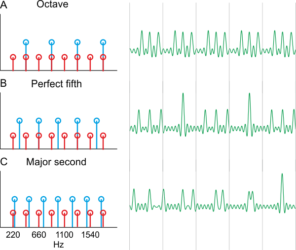
Figure 3.5
A (partial) theory of consonance. A schematic representation of the spectrum (left) and a portion of the waveform (right) of three combinations of two notes. The lower note is always an A on 220 Hz. Its harmonics are plotted in black and half height (left). The gray lines on the right mark the duration of one period of that lower note. (A) The higher note is A, an octave above the lower note. Its harmonics (gray full height) match a subset of the harmonics of the lower note, resulting in a sound whose periodicity is that of the lower note (the sound between each pair of successive gray lines is the same). (B) The higher note is E, a perfect fifth above A. The harmonics of this E are either midway or match exactly harmonics of the lower A. The waveform has a periodicity of 110 Hz (the pattern repeats every two gray lines on the right). (C) The higher note is B, a major second above A. None of the harmonics match and some of them are rather close to each other. The waveform doesn’t show any periodicity within the five periods that are displayed, and in fact its period is outside the existence region of pitch. It has irregular variations of amplitude (almost random location of the high peaks, with this choice of phases). This irregularity presumably results in the perception of dissonant sounds.
However, this theory does not readily explain consonance and dissonance of other intervals. For example, the interval of a perfect fourth, which corresponds to the frequency ratio of 4 to 3 (the ratio between the frequencies of the fourth and third harmonics), is considered as consonant, but would sound dissonant to many modern listeners. On the other hand, the interval of a major third was considered an interval to avoid in medieval music due to its dissonance, but is considered highly consonant in modern Western music. Thus, there is much more to consonance and dissonance than just the physics of the sounds.
All of this may appear rather arbitrary, and to some degree it is. However, the Western scale is really based on a rather natural idea that, when pushed far enough, results in inconsistencies. The formal system described above is the result of the development of this idea over a long period of time in an attempt to solve these inconsistencies, and it reached its final shape only in the nineteenth century.
Consider the C major key, with its seven pitch classes. What motivates the choice of these particular pitches, and not others? The Western scale is based on an interplay between the octave and the perfect fifth, which are considered to be the two most consonant intervals. (To remind the reader, the perfect fifth is the “ideal” interval between, e.g., C and G, with a ratio of 3 to 2, although we have seen that in current practice the fifth is slightly smaller.) The goal of the process we describe next is to create a set of notes that has as many perfect fifths as possible—we would like to have a set of pitches that contains a perfect fifth above and below each of its members. We will see that this is actually impossible, but let's start with the process and see where it fails.
Starting with C, we add G to our set of notes. Note that modern G is not a perfect fifth about C, but we will consider right now the “natural” G, which is. We are going to generate other notes which we will call by their modern names, but which are slightly different from their modern counterparts. The notes we are going to generate are the natural notes, so called because they are going generated by using jumps of natural fifths.
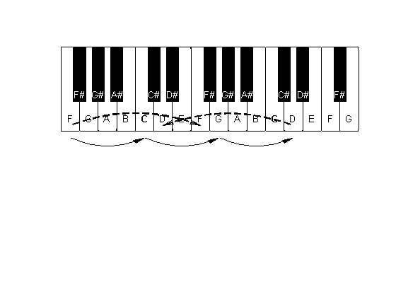
Figure 3.6
The beginning of the cycle of fifths. G is one fifth above C, and D (in the next octave) is one fifth above G. It is shifted down by an octave (dashed arrow). The fifth from F up to C is also displayed here, since F would otherwise not be generated (instead, E# is created as the penultimate step in the cycle, and the perfect 4/3 relationship with C would not exist). This F has to be shifted up by an octave in order to generate the F note within the correct range.
Since we want the scale to contain perfect fifths above and below each of its members, we also move one fifth down from C, to arrive at (natural) F, a note with an F0 of 2/3 that of C. This F is outside the octave starting at our C, so we move one octave up to get to the next higher F, which therefore has an F0 of 4/3 times that of the C that serves as our starting point. In this manner, we have already generated three of the seven pitch classes of the major scale, C, F, and G, just by moving in fifths and octaves (figure 3.6).
The other pitch classes of the major scale can be generated in a similar manner by continued use of perfect fifths and octaves. Moving from G up by one fifth, we get to natural D (at an interval of 3/2 × 3/2 = 9/4 above the original C). This interval is larger than an octave (9/4 > 2), however, and to get a tone in the original octave it has to be transposed by one octave down; in other words, its frequency has to be divided by 2. Thus, the natural D has a frequency that is 9/8 that of C. The next pitch class to generate is A, a perfect fifth above D (at a frequency ratio of 9/8 × 3/2 = 27/16 above C), and then E (at an interval of 27/16 × 3/2 = 81/32 above C). This is, again, more than an octave above C, and to get the E within the original octave, we transpose it down by an octave, arriving at an F0 for natural E, which is 81/64 that of C. Finally, a perfect fifth above E we get B, completing all the pitch classes of the major scale.
The scale that is generated using this interplay of fifths and octaves is called the natural, or Pythagorean, scale. The pitches of the natural scale are related to each other by ratios that are somewhat different from those determined by the equal-tempered chromatic scale we discussed previously. For example, the interval between E and C in the natural scale corresponds to a ratio of 81/64 » 1.266, whereas the corresponding interval of four semitones is 24/12 » 1.260. Similarly, the interval of a fifth corresponds to seven semitones, so in the modern scale it corresponds to a frequency ratio of 27/12 » 1.498, slightly smaller than 3/2 = 1.5. Why these differences?
We wanted to have a set of tones that contains the fifths above and below each of its members. We stopped at natural B, and we already generated the fifth below it (E), but not the fifth above it. So we have to continue the process. Moving up by perfect fifths and correcting by octaves, we generate next the five pitch classes that are still missing (in order F#, C#, G#, D#, and A#). However, thereafter the situation becomes less neat. The next pitch class would be E#, which turns out to be almost, but not quite, equal to F, our starting point (figure 3.6). This pitch class, the thirteenth tone in the sequence, has a F0, which is (3/2)12/27 times that of the original F—in other words, it is generated by moving up twelve times by a fifth and correcting seven times with an octave down. However, that frequency ratio is about 1.014 rather than 1. So, we generated twelve pitch classes using motions of fifths and octaves, but the cycle did not quite close at the thirteenth step.
Instruments can still be tuned by the natural scale, but then scales in keys that are far from C (along the cycle of fifths) do not have quite the right intervals, and therefore sound mistuned. On an instrument that is tuned for playing in the natural C major scale, music written in F# major will sound out of tune.
The problem became an important issue when, in the seventeenth and eighteenth centuries, composers started to write music in all keys, or even worse, started writing music that moved from one key to another within the same piece. To perform such music in tune, it was necessary to modify the natural scale. A number of suggestions have been made to achieve this. The modern solution consists of keeping octaves exact (doubling F0), but changing the definition of all other intervals. In particular, the interval of perfect fifth was abandoned for the slightly reduced modern approximation. As a result, twelve fifths became exactly seven octaves, and E# became exactly F. The resulting system fulfills our original goal of having a set of pitch classes in which we can go by a fifth above and below each of its members.
Is there any relationship between this story and the perceptual issues we discussed earlier? We encountered two such connections. The first is in the primacy of the octave and the fifth, the two most consonant intervals. The second is in the decision that the difference between E# and F was too small, and that the two pitch classes should be identified. Interestingly, essentially all formalized musical systems in the world use intervals of about the same size, with the smallest intervals being around half of the semitone. In other words, musical systems tend not to pack many more than twelve tones into the octave—maybe up to twenty-four, but not more than that. This tendency could possibly be traced to perceptual abilities. Music is a form of communication, and therefore requires distinguishable basic components. Thus, the basic steps of any musical scales should be substantially larger than the minimum discrimination threshold. It may well be that this is the reason for the quite constant density of notes in the octave across cultures. The specific selection of pitches for these notes may be justified by other criteria, but is perhaps more arbitrary.
3.5 Pitch Perception by Nonhuman Listeners
In order to study the way the nervous system estimates the pitch of sounds, we will want to use animal models. This raises a crucial issue: Is pitch special for humans, or do other species perceive pitch in a similar way? This is a difficult question. It is impossible to ask animals directly what they perceive, and therefore any answer is by necessity indirect. In spite of this difficulty, a number of studies suggest that many animals do have a perceptual quality similar to pitch in humans.
Thus, song birds seem to perceive pitch: European starlings (Sturnus vulgaris) generalize from pure tones to harmonic complexes with missing fundamental and vice versa. Cynx and Shapiro (1986) trained starlings to discriminate the frequencies of pure tones, and then tested them on discrimination of complex sounds with the same F0 but missing the fundamental. Furthermore, the complex sounds were constructed such that use of physical properties other than F0 would result in the wrong choice. For example, the mean frequency of the harmonics of the high-F0 sound was lower than the mean frequency of the harmonics of the low-F0 sound. As a result, if the starlings would have used place pitch instead of periodicity pitch, they would have failed the test.
Even goldfish generalize to some extent over F0, although not to the same degree as humans. The experiments with goldfish were done in a different way from those with birds. First, the animals underwent classical conditioning to a periodic sound, which presumably evokes a pitch sensation in the fish. In classical conditioning, a sound is associated with a consequence (a mild electric shock in this case). As a result, when the animal hears that sound, it reacts (in this case, by suppressing its respiration for a brief period). Classical conditioning can be used to test whether animals generalize across sound properties: The experimenter can present a different sound, which shares some properties with the original conditioning stimulus. If the animal suppresses its respiration, it is concluded that the animal perceives the new stimulus as similar to the conditioning stimulus. Using this method, Fay (2005) demonstrated some generalization—for example, the goldfish responded to the harmonic series in much the same way, regardless of whether the fundamental was present or missing. But Fay also noted some differences from humans. For example, IRNs, a mainstay of human pitch studies, do not seem to evoke equivalent pitch precepts in goldfish.
In mammals, it generally seems to be the case that “missing fundamentals are not missed” (to paraphrase Fay, 2005). Heffner and Whitfield (1976) showed this to be true in cats by using harmonic complexes in which the overall energy content shifted down while the missing fundamental shifted up and vice versa (a somewhat similar stratagem to that used by Cynx and Shapiro with starlings); and Tomlinson and Schwarz (1988) showed this in macaques performing a same-different task comparing sounds composed of subsets of harmonics 1–5 of their fundamental. The monkeys had to compare two sounds: The first could have a number of low-order harmonics missing while the second sound contained all harmonics.
Other, more recent experiments suggest that the perceptual quality of pitch in animals is similar but not identical to that evoked in humans. For example, when ferrets are required to judge whether the pitch of a second tone is above or below that of a first tone, their discrimination threshold is large—20% or more—even when the first tone is fixed in long blocks (Walker et al., 2009). Under such conditions, humans will usually do at least ten times better (Ahissar et al., 2006). However, the general trends of the data are similar in ferrets and in humans, suggesting the existence of true sensitivity to periodicity pitch.
Thus, animals seem to be sensitive to the periodicity, and not just the frequency components, of sounds. In this sense, animals can be said to perceive pitch. However, pitch sensation in animals may have somewhat different properties from that in humans, potentially depending more on stimulus type (as in goldfish) or having lower resolution (as in ferrets).
3.6 Algorithms for Pitch Estimation
Since, as we have seen, pitch is largely determined by the periodicity (or approximate periodicity) of the sound, the auditory system has to extract this periodicity in order to determine the pitch. As a computational problem, producing running estimates of the periodicity of a signal turns out to have important practical applications in speech and music processing. It has therefore been studied in great depth by engineers. Here, we will briefly describe some of the approaches that emerged from this research, and in a later section, we will discuss whether these “engineering solutions” correspond to anything that may be happening in our nervous systems when we hear pitch.
As discussed previously, there are two equivalent descriptions of the family of periodic sounds. The “time domain” description notes whether the waveform of the sound is composed of a segment of sound that repeats over and over, in rapid succession. If so, then the pitch the sound evokes should correspond to the length of the shortest such repeating segment. The “frequency domain” description asks whether the frequency content of the sound consists mostly or exclusively of the harmonics of some fundamental. If so, then the pitch should correspond to the highest F0 consistent with the observed sequence of harmonics. Correspondingly, pitch estimation algorithms can be divided into time domain and frequency domain methods. It may seem overcomplicated to calculate the frequency spectra when the sound waveform is immediately available, but sometimes there are good reasons to do so. For example, noise may badly corrupt the waveform of a sound, but the harmonics may still be apparent in the frequency domain. Possibly more important, as we have seen in chapter 2, the ear performs approximate frequency decomposition; therefore it may seem that a frequency domain algorithm might be more relevant for understanding pitch processing in the auditory system. However, as we will see later in this chapter, time domain methods certainly seem to play a role in the pitch extraction mechanisms used by the mammalian auditory system.
Let us first look at time domain methods. We have a segment of a periodic sound, and we want to determine its period. Suppose we want to test whether the period is 1 ms (F0 of 1,000 Hz). The thing to do would be to make a copy of the sound, delay the copy by 1 ms, and compare the original and delayed versions—if they are identical, or at least sufficiently similar, then the sound is periodic, with a period of 1 ms. If they are very different, we will have to try again with another delay. Usually, such methods start by calculating the similarity for many different delays, corresponding to many candidate F0s, and at a second stage select the period at which the correspondence between the original and delayed versions is best.
Alhtough this is a good starting point, there are many details that have to be specified. The most important one is the comparison process—how do we perform it? We will discuss this in some detail below, since the same issue reappears later in a number of guises. Selecting the best delay can also be quite complicated—several different delays may work quite well, or (not unusual with real sounds) many delays could be equally unsatisfactory. Algorithms often use the rule of thumb that the “best delay” is the shortest delay that is “good enough” according to some criteria that are tweaked by trial and error.
So, how are we to carry out the comparison of the two sounds (in our case, the original and delayed versions of the current bit of sound)? One way would be to subtract one from the other. If they are identical, the difference signal would be zero. In practice, however, the signal will rarely be strictly periodic, and so the difference signal would not be exactly zero. Good candidates for the period would be delays for which the difference signal is particularly small. So we have to gauge whether a particular difference signal is large or small. Just computing the average of the difference signal would not work, since its values are likely to be sometimes positive and sometimes negative, and these values would cancel when averaging. So we should take the absolute value of the differences, or square all differences, to make the difference signal positive, and then average to get a measure of its typical size.
There is, however, a third way of doing this comparison: calculating the correlation between the original and time-shifted signals. The correlation would be maximal when the time shift is 0 ms (comparing the sound with a nonshifted version of itself), and may remain high for other very small shifts. In addition, if the sound is periodic, the correlation will be high again for a time shift that is equal to the period, since the original sound and its shifted version would be very similar to each other at this shift. On the other hand, the correlation is expected to be smaller at other shifts. Thus, periodic sounds would have a peak in the correlation at time shifts equal to the period (or multiples thereof).
Although calculating the correlation seems a different approach from subtracting and estimating the size of the difference signal, the two approaches are actually closely related, particularly when using squaring to estimate the size of the difference signal. In that case, the larger the correlation, the smaller the difference signal would generally be.
While implementation details may vary, the tendency is to call all of these methods, as a family, autocorrelation methods for pitch estimation. The term “autocorrelation” comes from the fact that the comparison process consists of computing the correlation (or a close relative) between a sound and its own shifted versions. It turns out that biological neural networks have many properties that should enable them to calculate autocorrelations. Therefore, the autocorrelation approach is not a bad starting point for a possible neural algorithm. One possible objection against the use of autocorrelations in the brain stems from the delays this approach requires—since the lower limit of pitch is about 40 Hz, the correlation would require generating delays as long as 25 ms. That is a fairly long time relative to the standard delays produced by biological “wetware” (typical neural membrane time constants, conduction velocities, or synaptic delays would result in delays of a few milliseconds, maybe 10 ms), so how neural circuits might implement such long delay lines is not obvious. However, this potential problem can be overcome in various ways (de Cheveigné & Pressnitzer, 2006).
As we discussed previously, a different approach to the extraction of pitch would be to calculate the frequency content of the sound and then analyze the resulting pattern of harmonics, finding their largest common divisor. If we know the pattern of harmonics, there is a neat trick for finding their greatest common divisor. Suppose we want to know whether 1,000 Hz is a candidate F0. We generate a harmonic “sieve”—a narrow paper strip with holes at 1,000 Hz and its multiples. We put the frequency content of the sound through the sieve, letting only the energy of the frequency components at the holes fall through, and estimate how much of the energy of the sound successfully passed through the sieve. Since only harmonics of 1,000 Hz line up with these holes, if the sound has an F0 of 1,000 Hz, all of the energy of the sound should be able to pass through this sieve. But if the frequency composition of the sound is poorly matched to the structure of the sieve (for example, if there are many harmonics that are not multiples of 1,000 Hz), then a sizeable proportion of the sound will fail to pass through, indicating that another candidate has to be tested.
As in the autocorrelation method, in practice we start with sieves at many possible F0s (“harmonic hole spacing”), and test all of them, selecting the best. And again, as in the autocorrelation method, there are a lot of details to consider. How do we estimate the spectra to be fed through the sieves? As we discussed in chapters 1 and 2, the cochlea, while producing a frequency decomposition of a sound, does its calculations in fairly wide frequency bands, and its output may not be directly appropriate for comparison with a harmonic sieve, possibly requiring additional processing before the sieve is applied. How do we select the best candidate sieve out of many somewhat unsatisfactory ones (as would occur with real-world sounds)? How do we measure the amount of energy that is accounted for by each sieve? How “wide” should the holes in the sieve be? These issues are crucial for the success of an implementation of these methods, but are beyond the scope of this book. These methods are generally called harmonic sieve methods, because of the computational idea at their heart.
One major objection to harmonic sieve methods is that the harmonic sieve has to be assembled from a neural network somewhere in the brain, but it is not immediately obvious how such an object could be either encoded genetically or learned in an unsupervised manner. However, a natural scheme has recently been proposed that would create such sieves when trained with sounds that may not be periodic at all (Shamma & Klein, 2000). Thus, harmonic sieves for pitch estimation could, in principle, be created in the brain.
Let us see how the autocorrelation and the harmonic sieve approaches deal with a hard case. Consider a sound whose frequency components are 220, 320, and 420 Hz. This sound has a periodicity of 20 Hz, but evokes a pitch at 106 Hz: This is an example of a sound that evokes a pitch away from its F0.
How would the two approaches explain this discrepancy? Figure 3.7A displays two true periods (50 ms long) of this sound. Strictly speaking, the sound is periodic, with a period of 50 ms, but it has some repeating structure every somewhat less than 10 ms (there are ten peaks within the 100-ms segment shown). Indeed, figure 3.7B shows the autocorrelation function of this sound. It has a peak at a delay of 50 ms (not shown in figure 3.7B), corresponding to the exact periodicity of 20 Hz. But 20 Hz is below the lower limit of pitch perception, so we can safely assume that the brain does not consider such a long delay. Instead, the evoked pitch should correspond to a high correlation value that would occur at a shorter delay. Indeed, the highest correlation occurs at a delay of 9.41 ms. The delay of 9.41 ms corresponds to a pitch of 106 Hz. Autocorrelation therefore does a good job at identifying the correct pitch.
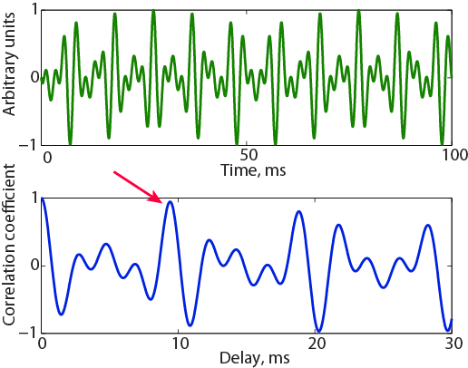
Figure 3.7
A sound composed of partials at 220, 320, and 420 Hz. The sound has a period of 50 ms (F0 of 20 Hz—two periods are displayed in the upper panel), which is outside the existence region for pitch. It evokes a low pitch at 106 Hz, which is due to the approximate periodicity at that rate (note the large peaks in the signal, which are almost, but not quite, the same). Indeed, its autocorrelation function (lower panel) has a peak at 9.41 ms (marked by the arrow).
How would the harmonic sieve algorithm account for the same result? As above, 20 Hz is too low for evoking a pitch. On the other hand, 106 Hz is an approximate divisor of all three harmonics: 220/106 = 2.07 (so that 220 Hz is almost the second harmonic of 106 Hz), 320/106 = 3.02, and 420/106 = 3.96. Furthermore, 106 is the best approximate divisor of these three numbers. So the harmonic sieve that best fits the series of frequency components corresponds to a pitch of 106 Hz. This example therefore illustrates the fact that the “holes” in the sieve would need to have some width in order to account for perception!
3.7 Periodicity Encoding in Subcortical Auditory Pathways
We have just seen how one might try to program a computer to estimate the pitch of a sound, but is there any relationship between the engineering methods just discussed and what goes on in your auditory system when you listen to a melody? When discussing this issue, we have to be careful to distinguish between the coding of periodicity (the physical attribute) and coding of pitch (the perceptual quality). The neural circuits that extract or convey information about the periodicity of a sound need not be the same as those that trigger the subjective sensation of a particular pitch. To test whether some set of neurons has any role to play in extracting periodicity, we need to study the relationship between the neural activity and the sound stimuli presented to the listener. But if we want to know what role that set of neurons might play in triggering a pitch sensation, what matters is how the neural activity relates to what the listeners report they hear, not what sounds were actually present. We will mostly discuss the encoding for stimulus periodicity, and we briefly tackle the trickier and less well understood question of how the sensation of pitch is generated in the next section.
Periodicity is encoded in the early stations of the auditory system by temporal patterns of spikes: A periodic sound would elicit spike patterns in which many interspike intervals are equal to the period of the sound (we elaborate on this statement later). It turns out that some processes enhance this representation of periodicity in the early auditory system, increasing the fraction of interspike intervals that are equal to the period. However, this is an implicit code—it has to be “read” in order to extract the period (or F0) of the sound. We will deal with this implicit code first.
The initial representation of sounds in the brain is in the activity of the auditory nerve fibers. We cannot hope that periodicity (and therefore pitch) would be explicitly encoded by the firing of auditory nerve fibers. First, auditory nerve fibers represent frequency content (as we discussed in chapter 2), and the relationships between frequency content and periodicity are complex. Furthermore, auditory nerve fibers carry all information needed to characterize sounds, including many dimensions other than pitch. Therefore, the relationship between pitch and the activity pattern of auditory nerve fibers cannot be straightforward.
Nevertheless, the activity pattern of auditory nerve fibers must somehow carry enough information about the periodicity of sounds so that at some point brain circuits can extract the pitch. Understanding how periodicity is encoded in the activity of auditory nerve fibers is therefore important in order to understand how further stations of the nervous system would eventually generate the pitch percept.
The key to understanding encoding of periodicity in the auditory nerve is the concept of phase locking—the tendency of fibers to emit spikes at specific points during each period, usually corresponding to amplitude maxima of the motion of the basilar membrane (see chapter 2). As a result, a periodic waveform creates a pattern of spike times that repeats itself (at least on average) on every period of the sound. Thus, the firing patterns of auditory nerve fibers in response to periodic sounds are themselves periodic. If we can read the periodicity of this pattern, we have F0. As usual, there are a lot of details to consider, the most important of which is that auditory nerve fibers are narrowly tuned; we will consider this complexity later.
How do we find the periodicity of the auditory nerve fiber discharge pattern? When we discussed algorithms for estimating periodicity, we developed the idea of autocorrelation—a process that results in an enhanced representation of the periodicity of a waveform. The same process can be applied to the firing patterns of auditory nerve fibers. Since the waveform of neuronal firings is really a sequence of spikes, the autocorrelation process for auditory nerve fibers has a special character (figure 3.8). This process consists of tallying the number of time intervals between each spike and every other spike in the spike train. If the spike train is periodic, the resulting interval histogram will have a strong representation of the interval corresponding to the period: Many spikes would occur at exactly one period apart, whereas other intervals will be less strongly represented.
The autocorrelation in its pure form is not a very plausible mechanism for extracting periodicity by neurons. For one thing, F0 tends to vary with time—after all, we use pitch to create melodies—and, at least for humans, the range of periods that evoke pitch is limited. Therefore, using all intervals in a long spike train does not make sense. Practical algorithms for extracting periodicity from auditory nerve firings would always limit both the range of time over which they tally the interspike intervals, and the range of intervals they would consider as valid candidates for the period.
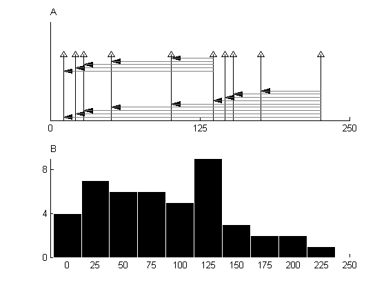
Figure 3.8
Autocorrelation of a spike sequence containing two approximate repeats of the same spike pattern at an interval of 125 ms. (A) The autocorrelation is a tally of all intervals between pairs of spikes. This can be achieved by considering, for each spike, the intervals between it and all preceding spikes (these intervals are shown for two of the spikes). (B) The resulting histogram. The peak at 125 ms corresponds to the period of the spike pattern in A.
What would be reasonable bounds? A possible clue is the lower limit of pitch, at about 40 Hz. This limit suggests that the auditory system does not look for intervals that are longer than about 25 ms. This might well be the time horizon over which intervals are tallied. Furthermore, we need a few periods to perceive pitch, so the duration over which we would have to tally intervals should be at least a few tens of milliseconds long. While the lower limit of pitch would suggest windows of ~100 ms, this is, in fact, an extreme case. Most pitches that we encounter are higher—100 Hz (a period of 10 ms) would be considered a reasonably deep male voice—and so a 40 ms long integration time window may be a practical choice (the window may even be task dependent).
The shortest interval to be considered for pitch is about 0.25 ms (corresponding to a pitch of 4,000 Hz). This interval also poses a problem—auditory nerve fibers have a refractory period of about 1 ms, and anyway cannot fire at sustained rates that are much higher than a few hundred Hertz. As a result, intervals as short as 0.25 ms cannot be well represented in the firings of a single auditory nerve fibers. To solve this problem, we would need to invoke the volley principle (chapter 2): We should really consider the tens of auditory nerve fibers that innervate a group of neighboring inner hair cells, and calculate the autocorrelation of their combined spike trains.
Until this point, we have considered a single nerve fiber (or a homogeneous group of fibers with the same CF), and assumed that the periodicity of the sound is expressed in the firing of that particular fiber. However, this is usually wrong! In fact, many periodic sounds contain a wide range of frequencies. On the other hand, auditory nerve fibers are narrowly tuned—as we have seen in chapter 2, they respond only to a restricted range of frequencies, even if the sound contains many more frequencies. As a specific example, consider the sound consisting of frequency components at 200, 400, and 600 Hz. This sound has an F0 of 200 Hz, and, at moderate sound levels, it would evoke activity mostly in auditory nerve fibers whose characteristic frequencies are near its component frequencies. Thus, an auditory nerve fiber responding to 200 Hz would be activated by this sound. The bandwidth of the 200-Hz auditory nerve fiber would be substantially less than 200 Hz (in fact, it is about 50 Hz, based on psychophysical experiments). Consequently it would “see” only the 200-Hz component of the sound, not the higher harmonics. We would therefore expect it to fire with a periodicity of 200 Hz, with a repetition of the firing pattern every 5 ms, corresponding to the correct F0. In a similar way, however, the 400-Hz auditory nerve fiber would respond only to the 400-Hz component of the sound, since its bandwidth would be substantially less than 200 Hz (about 60 Hz). And because it phase locks to a harmonic, not to the fundamental, it would fire with a periodicity of 400 Hz, with a repetition of the firing pattern every 2.5 ms, which corresponds to a wrong periodicity.
The same problem would not occur for higher harmonics. To continue with the same example, the bandwidth of the auditory nerve fibers whose best frequency is 2,000 Hz in humans is believed to be larger than 200 Hz. As a result, if our sound also included harmonics around 2,000 Hz (the tenth harmonic of 200 Hz), auditory nerve fibers around that frequency would hear multiple harmonics. A sound composed of multiple harmonics of 200 Hz would have a periodicity of 200 Hz, and therefore the 2,000-Hz auditory nerve fibers would have a periodic firing pattern with a periodicity of 200 Hz.
This difference between lower and higher harmonics of periodic sounds occurs at all pitch values, and it has a name: The lower harmonics (up to order 6 or so) are called the resolved harmonics, while the higher ones are called unresolved. The difference between resolved and unresolved harmonics has to do with the properties of the auditory system, not the properties of sounds—it is determined by the bandwidth of the auditory nerve fibers. However, as a consequence of these properties, we cannot calculate the right periodicity from the pattern of activity of a single auditory nerve fiber in the range of resolved harmonics. Instead, we need to combine information across multiple auditory nerve fibers. This can be done rather easily. Going back to the previous example, we consider the responses of the 200-Hz fiber as “voting” for a periodicity of 5 ms, by virtue of the peak of the autocorrelation function of its spike train. The 400-Hz fiber would vote for 2.5 ms, but its spike train would also contain intervals of 5 ms (corresponding to intervals of two periods), and therefore the autocorrelation function would have a peak (although possibly somewhat weaker) at 5 ms. The autocorrelation function of the 600-Hz fiber would peak at 1.66 ms (one period), 3.33 ms (two periods), and 5 ms (corresponding to intervals between spikes emitted three periods apart). If we combine all of these data, we see there is overwhelming evidence that 5 ms is the right period.
The discussion we have just gone through might suggest that the pitch of sounds composed of unresolved harmonics may be stronger or more robust than that of sounds composed of resolved harmonics, which requires across-frequency processing to be extracted. It turns out that exactly the opposite happens—resolved harmonics dominate the pitch percept (Shackleton & Carlyon, 1994), and the pitch of sounds composed of unresolved harmonics may not correspond to the periodicity (as demonstrated with Sound Example "Pitch of 3-Component Harmonic Complexes" on the book's Web site ). Thus, the across-frequency integration of periodicity information must be a crucial aspect of pitch perception.
A number of researchers studied the actual responses of auditory nerve fibers to stimuli-evoking pitch. The goal of such experiments was to test whether all the ideas we have been discussing work in practice, with real firing of real auditory nerve fibers. Probably the most complete of these studies were carried by Peter Cariani and Bertrand Delgutte (Cariani & Delgutte, 1996a, b). They set themselves a hard problem: to develop a scheme that would make it possible to extract pitch of a large family of pitch-evoking sounds from real auditory nerve firings. To make the task even harder (but closer to real-life conditions), they decided to use stimuli whose pitch changes with time as well.
Figure 3.9 shows one of the stimuli used by Cariani and Delgutte (Sound Example "Single Formant Vowel with Changing Pitch" on the book's Web site <flag>). At each point in time, it was composed of a sequence of harmonics. The fundamental of the harmonic complex varied continuously, initially going up from 80 to 160 Hz and then back again (figure 3.9C). The amplitudes of the harmonics varied in time so that the peak harmonic always had the same frequency (at low F0, the peak amplitude occurred at a higher-order harmonic, whereas at high F0 it occurred at a lower-order harmonic; this is illustrated in figure 3.9A and B). The resulting time waveform, at a very compressed time scale, is shown in figure 3.9D. For reasons that may become clear in chapter 4,[DH1] this stimulus is called a single formant vowel.
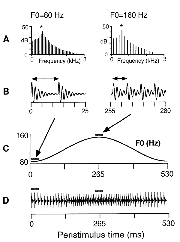
Figure 3.9
The single-formant vowel stimulus with varying pitch used by Cariani and Delgutte. (A) Spectra of the stimulus at its beginning (pitch of 80 Hz) and at its middle (pitch of 160 Hz). At the lower pitch, the harmonics are denser (with a separation of 80 Hz) and at the higher pitch they are less dense (with a separation of 160 Hz). However, the peak amplitude is always at 640 Hz. (B) The time waveform at the beginning and at the middle of the sound, corresponding to the spectra in A. At 80 Hz, the period is 12.5 ms (two periods in the 25-ms segment displayed in the figure), while at 160, the period is 6.25 ms, so that in the same 25 ms there are four periods. (C) The pattern of change of the F0 of the stimulus. (D) The time course of the stimulus, at a highly compressed time scale. The change in pitch is readily apparent as an increase and then a decrease in the density of the peaks.
Cariani and Delgutte recorded the responses of many auditory nerve fibers, with many different best frequencies, to many repetitions of this sound. They then used a variant of the autocorrelation method to extract F0. Since F0 changed in time, it was necessary to tally intervals separately for different parts of the stimulus. They therefore computed separate autocorrelation functions for 20-ms sections of the stimulus, but overlapped these 20-ms sections considerably to get a smooth change of the autocorrelation in time. In order to integrate across many frequencies, Cariani and Delgutte did almost the simplest thing—they added the time-varying autocorrelation patterns across all the auditory nerve fibers they recorded, except that different frequency regions were weighted differentially to take into account the expected distribution of CFs.
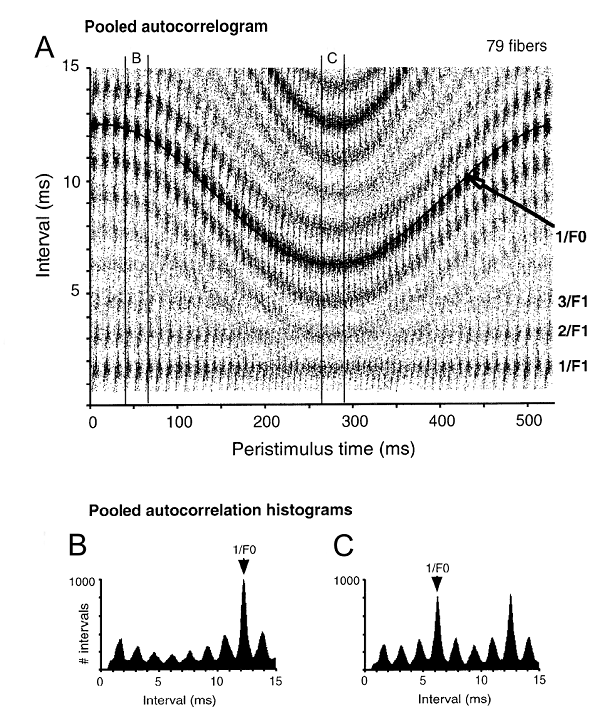
Figure 3.10
(A) The time-varying autocorrelation function of Cariani and Delgutte. Time during the stimulus is displayed along the abscissa. At each time along the stimulus, the inter-spike intervals that occurred around that time as tallied and the histogram are displayed along the ordinate. This process was performed for segments of 20 ms, with a substantial amount of overlap. (B) A section of the time-varying autocorrelation function, at the beginning of the sound. Note the single high peak at 12.5 ms. (C) A section of the time-varying autocorrelation function, at the time of the highest pitch. There are two equivalent peaks, one at the correct period and one at twice the period.
The rather complex result of this process is displayed in figure 3.10A. Time through the stimulus is represented along the abscissa, interval durations are along the ordinate, and the values of the time-varying autocorrelation function are displayed in gray level. Let us focus our attention on the abscissa at a certain time (e.g., the small window around 50 ms, marked in figure 3.10A by the two vertical lines with the “B” at the top). This strip is plotted in details in figure 3.10B. This is the autocorrelation function around time 50 ms into the stimulus: the tally of the interspike intervals that occurred around this time in the auditory nerve responses. Clearly, these interspike intervals contain an overrepresentation of intervals around 12.5 ms, which is the pitch period at that moment. Figure 3.10C shows a similar plot for a short window around time 275 ms (when the pitch is highest, marked again in figure 3.10A by two vertical lines with “C” at the top). Again, there is a peak at the period (6.25 ms), although a second peak at 12.5 ms is equal to twice the period. This is one of those cases where it is necessary to make the correct decision regarding the period: Which of these two peaks is the right one? The decision becomes hard if the peak at the longer period is somewhat larger than the peak at the shorter period (for example, because of noise in the estimation process). How much larger should the longer period peak be before it is accepted as the correct period? This is one of the implementation questions that have to be solved to make this process work in practice.
The resulting approach is surprisingly powerful. The time-varying period is tracked successfully (as illustrated by the high density of intervals marked by 1/F0 in figure 3.10A). Cariani and Delgutte could account not only for the estimation of the time-varying F0, but also for other properties of these sounds. Pitch salience, for example, turns out to be related to the size of the autocorrelation peak at the perceived pitch. Larger peaks are generally associated with stronger, or more salient, pitch.
The major conclusion from studies such as that of Cariani and Delgutte is that it is certainly possible to read F0 from the temporal structure of auditory nerve fiber responses, so there is no magic here—all the information necessary to generate the pitch percept is available to the brain. On the other hand, these studies do not tell us how the brain extracts periodicity or generates the percept of pitch; for that purpose, it is necessary to go higher up into the auditory system.
The auditory nerve fibers terminate in the cochlear nucleus. The cochlear nucleus has multiple cell types, transforming the representation of sounds in the auditory nerve arrays in various ways (chapter 2). When testing these neurons with pitch-evoking stimuli, Ian Winter and his colleagues (2001) found that, as in the auditory nerve, the autocorrelation functions of these neurons have an overrepresentation of the pitch period. However, some of these neurons show an important variation on this theme: The representation of the pitch period was also enhanced in their first-order intervals (those between one spike and the following one). Extracting the periodicity of the sound from the activity of these neurons is therefore easier than extracting it from auditory nerve fibers: Whereas calculating autocorrelations requires measuring all intervals, including those that contain other spikes, counting first-order intervals requires only measuring the times from one spike to the next.
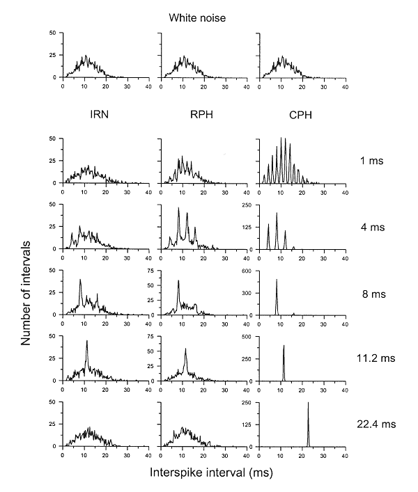
Figure 3.11
First-order interspike intervals of an onset chopper unit in response to noise and to three types of pitch-evoking stimuli with different periods. The first-order intervals are those between a spike and the next one, rather than intervals of all order (as in figure 3.8). This unit represents well periods of 8 ms and 11.2 ms, with weaker representation of shorter and longer periods.
From figure 5 in Winter, Wiegrebe, and Patterson (2001).
Figure 3.11 illustrates this effect. First-order interspike interval histograms are displayed for an “onset-chopper neuron,” one type of neuron found in the ventral cochlear nucleus (VCN). The neuron fires rather regularly even when stimulated with irregular stimuli such as white noise—its interspike intervals have a clear peak at about 10 ms. The neuron was tested with three types of stimuli that evoke pitch: IRN, random phase harmonic complexes (RPH, as in figure 3.1C), and cosine phase harmonic complexes (CPH; these are periodic sounds with a single large peak in their period). CPHs are often used as pitch-evoking stimuli, but they are in a sense extreme. Indeed, in response to CPHs, the neuron fired almost exclusively at the pitch period and its multiples—its spikes were apparently very strongly locked to the large-amplitude peak that occured once during each period of the stimulus. The more interesting tests are therefore the other two stimuli, which do not contain the strong temporal envelope cues that occur in the CPH. For these two stimulus types, the interspike interval histograms sometimes contained a sharp peak at the stimulus period. This occured most clearly when the pitch period was close to 10 ms, which also happened to be the preferred interval for this neuron when stimulated by white noise. Thus, this neuron enhances the representation of the periodicity of pitch-evoking stimuli around its preferred interval.
This turns out to be a rather general finding—many cell types in the cochlear nucleus show such interval enhancement, and for many of them the preferred first-order interspike interval can be observed, for example, in the neuron’s response to white noise. The range of best intervals of neurons in the cochlear nucleus is rather wide, covering at least the range from 1 to 10 ms and beyond (1,000 Hz to below 100 Hz).
As we mentioned earlier, the perceived pitch of a sound tends to change very little with change in sound levels. However, many response properties of neurons in the more peripheral parts of the auditory system depend very strongly on sound level. For example, the preferred intervals of onset choppers in the VCN become shorter with increasing sound level—this is related to the high firing rates of those neurons in response to white noise. Thus, although onset choppers represent periodicity well, they prefer different best periodicities at different sound levels. This makes the readout of the periodicity information from their responses complicated (although not impossible).
However, it turns out that one type of neurons in the VCN, the so-called sustained choppers, shows both an enhancement of the representation of periodicity by first-order interspike intervals and preferred intervals, which are essentially independent of sound level. These neurons could be the beginning of a pathway that encodes periodicity in a level-invariant way.
Thus, at the output of the cochlear nucleus, we have neurons that strongly represent F0 in their temporal firing pattern. This is still not an explicit representation of F0—we only made it easier for a higher station to extract F0. In terms of the algorithms we discussed earlier, the all-interval autocorrelation process can be replaced by a simple tallying of the first-order intervals between spikes. While this substantially facilitates the computational problem facing the next stations of the auditory pathways, the crucial step, which is calculating the periodicity itself, has apparently not yet been performed in the VCN.
The cochlear nucleus projects both directly and indirectly to the inferior colliculus (IC). At the level of the IC, the representation of periodicity in terms of the temporal firing patterns appears to be transformed into a firing rate code. IC neurons generally appear less able to phase lock to particular periods with the same vigor and precision as neurons in the VCN. Instead, some neurons in the IC appear to be tuned to specific periodicities—one of these neurons might, for example, respond with high firing rates to sounds with a period of 100 Hz and not respond at all to sounds with a period of 10 Hz or 1,000 Hz (figure 3.12A). An array of such neurons could, in principle, encode periodicity in the same way that the array of auditory nerve fibers encodes frequency content. If this array of “periodicity tuned neurons” was arranged in a systematic manner, the result would be a “periodotopic map” (Schreiner & Langner, 1988). However, many results argue against such an explicit, topographic representation of periodicity in IC.
Figure 3.12 shows the responses of two IC neurons to amplitude-modulated BF tones presented with varying sound levels. These stimuli evoke relatively weak pitch (if at all), but nevertheless have been extensively used to study the coding of periodicity in the IC. The modulation frequency (represented along the abscissa) would correspond to the evoked pitch. Figure 3.12A shows the responses of a classical neuron—it has a best modulation frequency at about 60 Hz, and its response at all modulation frequencies grows monotonically with level.
Figure 3.12
The responses of two IC neurons to periodic sounds (SAM complexes). (A) This neuron responds to a narrow range of periods, centered at 60 Hz, and increases monotonically its firing rate with increased sound level (different symbols). (B) This neuron has a complex pattern of responses as a function of period and sound level.
From figures 5 and 6 in Krishna and Semple (2000).[dh2]
However, such neurons are not necessarily typical of IC. Most neurons do not have a clear preference for specific modulation rates. Figure 3.12B shows the responses of another neuron. This neuron had a complex pattern of responses as a function of sound level: At low levels it responded weakly with a peak around 100 Hz (filled circles), at intermediate levels it responded to all modulation frequencies without significant selectivity (open squares), and at high sound levels it failed to respond to a restricted set of modulation frequencies while responding to all others (stars, filled triangles, and open diamonds). Thus, a first objection against the presence of a periodotopic map in IC is the finding that IC neurons are far from uniform in their responses to modulation frequencies, and their selectivity to periodic stimuli sometimes depends on irrelevant variables such as sound level. This objection could be surmounted by positing that the representation of the periodicity map is really the role of the classical neurons, excluding the neurons with more complex response patterns.
Another major problem with the assumption that a periodotopic map in IC might serve as a neural substrate for pitch perception is that the range of preferred modulation frequencies (and hence, stimulus periods) found in the IC does not correspond to the range of perceived pitches. In a number of species in which these issues have been tested (including cats, gerbils, guinea pigs, and chinchillas), the large majority of IC neurons responds maximally to modulation frequencies below 100 Hz, with a small number of exceptions. Thus, the “pitch axis” would be represented far from uniformly (remember that the note middle A, about the middle of the musical pitch range in humans, has a frequency of 440 Hz), and neurons capable of representing pitch in this manner in the kilohertz range would be very rare, indeed.
Figure 3.13
A cosine-phase harmonic complex (upper panel) and an alternating-phase harmonic complex (lower panel). In each panel, the waveform is plotted in black, and the envelope in gray. IC neurons respond to the envelope periodicity, and therefore respond to an alternate-phase complex as if it had half the period of the corresponding cosine-phase complex.
Finally, more refined tests of pitch selectivity in the IC suggest that the selectivity to periodicity of IC neurons may have nothing to do with pitch. Surprisingly, few studies have tested IC neurons with periodic stimuli that evoke a strong pitch percept. Those that have been conducted suggest that IC neurons are sensitive to the periodicity in the envelope of sounds. To see why this is important, consider the sounds in figure 3.13. Both sounds have a period of 10 ms, evoking a pitch of 100 Hz (Sound Example "Periodicity of Sounds and of Envelopes" on the book's Web site). Figure 3.13A displays the waveform of a sound with a single prominent peak in each period, but figure 3.13B displays the waveform of a sound with two prominent peaks in each period (one positive and one negative). Gray lines display the envelope of the two sounds, which measures the overall energy at each moment in time. The envelope of the sound in figure 3.13B has a period of 5 ms, because of the presence of the second peak. When played to IC neurons, sounds such as the one in figure 3.13B evoke responses that correspond to the periodicity of its envelope, rather than to its true periodicity (Shackleton, Liu, & Palmer, 2009).
Thus, the relationship between the representation of periodicity in the IC and pitch is still unclear. It may well be that there is a subset of IC neurons that do encode waveform periodicity, rather than envelope periodicity, but these have not been demonstrated yet.
3.8 Periodicity Coding in Auditory Cortex
Is there an “explicit” representation of periodicity in the auditory system? It may seem strange to raise this question now, after we have been putting much effort into discussing how pitch might be extracted and represented. But the question is not trivial at all. We cannot exclude the possibility that periodicity is represented only implicitly in the auditory system, in the sense that neural responses in the auditory pathway might never fully separate periodicity from other physical or perceptual qualities of a sound, such as intensity, timbre, or sound source direction. Such an “implicit” representation would not necessarily make it impossible for other, not strictly auditory but rather cognitive or motor areas of the brain to deduce the pitch of a sound if the need arises (similar arguments have been made in the context of so-called motor theories of speech perception).
There is, however, some evidence from imaging experiments (Krumbholz et al., 2003) that parts of the auditory cortex may respond in a “periodicity specific” manner. This experiment used noise stimuli, which metamorphosed from simple, pitchless noise to pitch-evoking but otherwise acoustically similar IRNs (as in figure 3.3B). The transition between noise and IRNs was controlled so that there was no change in bandwidth or sound level. These sounds were played to subjects while the magnetic fields from their brains were recorded. The magnetic fields showed a transient increase just past the change point, resulting in what the authors called pitch onset responses (PORs). These responses increased with pitch strength (related to the number of iterations used to generate the IRNs) and shifted in time with the period—it seems as if the brain had to count a fixed number of periods before it generated the PORs. Finally, MEG recordings allow some level of localization of the currents that create the fields, and the source of the POR seems to be in auditory cortex (although not necessarily in primary auditory cortex). These results show that human auditory cortex takes notice when periodicity appears or disappears in the ongoing soundscape, but they do not tell us much about how periodicity is represented there.
Before we delve deeper into recent experiments that have tried to shed light on cortical representations of pitch, let us briefly consider what properties such a cortical representation might have. We expect neurons that participate in such representation to be sensitive to periodicity—they should respond to periodic sounds and not (or less) to nonperiodic sounds. We expect their responses to be somehow modulated by periodicity—their rate, or their firing patterns, should be different for different F0s. These properties are necessary since periodicity is the primary correlate of pitch. In particular, properties such as sound level, timbre, or spatial location should not affect the responses of these neurons, or should affect them in ways that do not impact on their ability to encode periodicity.
However, these properties miss an important feature of pitch—that it is a perceptual, rather than physical, property of sounds. The crucial property of a true pitch representation (in addition to its representation of periodicity) is that it should be able to underpin the listener’s perception of pitch. This last, and perhaps most problematic, requirement harks back to a point we made in the opening paragraphs of this chapter, when we pondered the ANSI definition of pitch as an “attribute of sound” that enables listeners to “order sounds on a scale from high to low.” If a cortical representation is to underpin the listener’s perception, then properties of stimulus-response relationships, such as those we just discussed, are insufficient. Since pitch is a perceptual phenomenon, it is what the listener thought he or she heard, not what the sound actually was, that really matters. A cortical representation of pitch therefore ought to reflect the listener’s subjective experience rather than the actual sound. For example, such pitch representation ought to discriminate between pitch values no worse, but also no better, than the listener. Even more important, when asked to make difficult pitch judgments, it should make the same mistakes as the listener on each and every trial.
There is one more property that a pitch representation may have (but is not required to have), and which would make it much easier to find it. Ever since Paul Broca’s (who we will meet again in chapter 4) description of cortical speech area in the 1860s, scientists have been fond of the idea that particular functions might be carried out by neatly localized cortical modules. Such a cortical pitch module would be particularly neat if it featured a topographic (periodotopic) map. However, the existence of a specialized pitch area, or indeed of a topographic pitch map within it, is by no means a necessity, as one could also envisage a distributed cortical pitch network whose constituent neurons were spread out over potentially a wide area and interspersed with neurons that carry out functions other than pitch analysis. Such a distributed arrangement would look messy to the investigator, but might bring advantages to the brain, such as improved fault tolerance (there are, for example, few cases of selective pitch deficits following strokes or small lesions to the brain) or improved interactions between pitch and nonpitch representations for auditory streaming or object recognition.
A number of studies have looked for putative pitch representations in the cortex of humans as well as other mammals, using either electrophysiological recordings or functional imaging methods. It is not uncommon for particular brain regions identified in these studies to be referred to as “pitch centers.” However, we deliberately try to avoid this: To demonstrate that a cortical region is indeed a pitch center, showing that it responds selectively to sounds that evoke pitch is not enough. One would also need to demonstrate that it is playing an important role in shaping the listener’s subjective pitch percept, and, to date, no study has fully achieved that, although they have provided some interesting pieces of the puzzle. We will review first the single neuron evidence.
In primary auditory cortex, there appears to be no explicit and invariant representation of stimulus periodicity. There are by now a fair number of studies that failed to demonstrate pure sensitivity to periodicity in single neurons of primary auditory cortex, in a number of species, including cats and macaques (Qin et al., 2005; Schwarz & Tomlinson, 1990). But if primary auditory cortex does not represent periodicity explicitly, higher-order cortical fields might.
The best evidence to date for neurons that might be specifically sensitive to periodicity is in a nonprimary area of the marmoset auditory cortex. This area, studied by Bendor and Wang (2005), lies adjacent to the low-frequency area of primary auditory cortex but seems to be distinct from it. Some neurons in this area respond equally well to pure tones of some particular frequency and to harmonic complexes made up of multiples of that frequency but with a missing fundamental. Thus, these neurons appear to be specifically interested in stimulus periodicity, rather than responding merely to sound energy at F0.
Figure 3.14 illustrates these responses. The neuron was tested with complexes consisting of three harmonics of 200 Hz up to high harmonic numbers (figure 3.14A). It responded to all of these complexes, although its responses decreased somewhat at very high harmonic numbers (figure 3.14B). The neuron also responded to pure tones around the same frequency (figure 3.14C), but its tuning was narrow enough that it didn't respond to any of the other harmonics of 200 Hz when presented by itself (figure 3.14E).
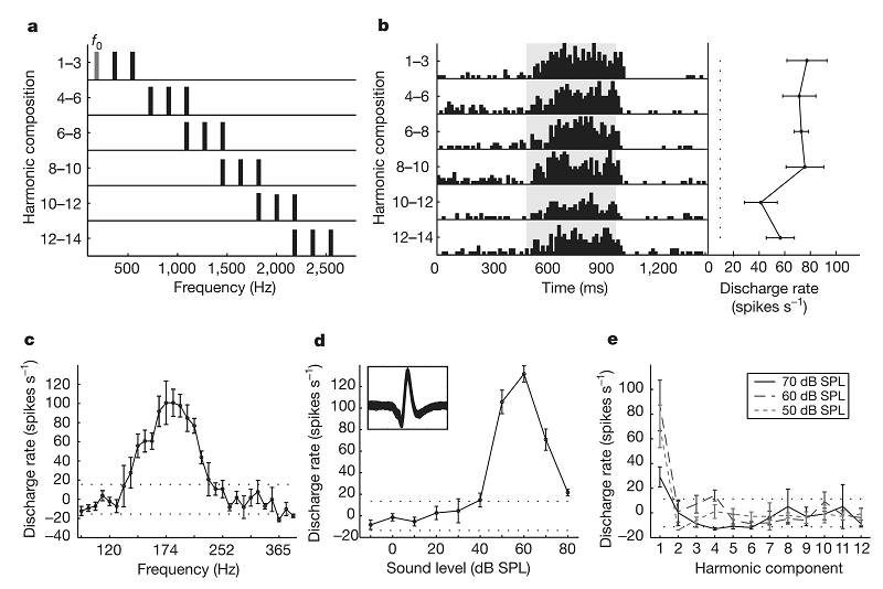
Figure 3.14
(A) Schematic representation of the stimuli used by Bendor and Wang, consisting of three successive harmonics with harmonic numbers from 1 to 14. (B) Responses of a neuron to these harmonic complexes. (C) Responses of the same neuron to pure tones, showing a narrow tuning centered on 200 Hz. (D) Response of this neuron as a function of level. The neuron did not response to a 200-Hz tone below the level of 40 dB SPL. (E) Responses to pure tones at the harmonic frequencies at three levels, showing that responses to pure sine waves occurred only to the first harmonic of the complexes in A.
From figure 1 in Bendor and Wang (2005).
While these data suggest that this neuron is, indeed, sensitive to the periodicity of the stimuli in figure 3.14A, such neurons have to pass two control to be able to say with certainty that they qualify as bona fide periodicity-selective neurons. The first is to be able to generalize to other periodic stimuli. The second, and possibly harder control to perform, is to exclude the possibility that the neuron might really respond to combination tones that are generated by nonlinearities in the cochlea. As we had seen in chapter 2, section 2.3, combination tones are cochlear responses at frequencies that are sum and differences of the tone frequencies that compose the sound. The two main combination tones in the cochlea are f2–f1 (the difference between the frequency of the higher and lower tones) and 2f1–f2. It is therefore quite possible that the three-component harmonic complexes used by Bendor and Wang could generate combination tones at F0. In other words, the cochlea might reinstate the missing fundamental, and the neurons, rather than being truly periodicity sensitive even in the absence of the fundamental, might simply be driven by the cochlear combination tone. Bendor and Wang tried to control for combination tones by using relatively low-level sounds, hoping that this would keep the amplitude of the combination tones too small to excite the neurons they investigated. How effective this was at keeping combination tones out of the picture is difficult to know. These controls are important since there is good evidence that pitch does not depend on combination tones. One example we encountered is the complex of 220, 320, and 420 Hz. This complex would create a cochlear combination tone at 100 Hz, but its pitch is 106 Hz, one semitone higher. So, while the neurons described by Bendor and Wang are the best candidates to date for encoding periodicity, they require a substantial amount of study to confirm them in this role.
Even if these neurons encode periodicity, their role as “pitch neurons” remains uncertain, chiefly because so far no evidence indicates that these neurons play a key role in generating or informing the animal’s subjective pitch perception. If pitch neurons are really anatomically clustered in a small region, as Bendor and Wang suspect, investigating their role in perception would be relatively easier, because it would then be possible to combine behavioral studies to measure subjective pitch judgments with electrophysiological recording, microstimulation, or lesion studies.
The evidence from other animal experiments is conflicting. A number of studies tried to probe periodicity coding in cortex by imaging of intrinsic optical signals related to blood oxygenation and blood flow. In an influential study, Schulze and colleagues (2002) obtained data suggesting that a periodotopic map overlies the frequency map in A1 of gerbils, although with a different orientation. However, these experiments were carried out using sounds that do not evoke pitch in humans (when properly controlled for combination tones): high-frequency tones that were sinusoidally amplitude modulated with low-frequency envelopes (SAM tones). Other periodic sounds were not used, so we do not know whether the map identified is capable of representing the periodicity of different stimulus types in a similar, consistent manner. To investigate this, we have repeated these experiments in ferrets (Nelken et al., 2008), and though we did observe topographically organized periodicity sensitivity using the same SAM tones, these maps did not generalize to other periodic stimuli. Our experiments failed to find any consistent periodotopic representation in either in A1 of the ferret or the immediately adjacent secondary cortical fields, including areas that would correspond to the periodicity representation suggested by Bendor and Wang in marmosets.
It is possible, of course, perhaps even likely, that significant species differences may exist between marmosets, ferrets, and gerbils, so it is hard to be certain to what extent results obtained in these species are indicative of mammalian auditory cortex in general. Furthermore, one may wonder whether optical imaging techniques, which after all rely on rather indirect measures of neural activity, are actually sensitive enough to reveal a true picture of the underlying functional organization of cortex. In the light of the experimental data available to date, however, many researchers remain sceptical about the existence of periodotopic maps in mammalian cortex that could represent pitch topographically.
Since we don't seem to be able to get a hold on periodotopic maps, can we at least identify a region of cortex that appears particularly responsive to stimulus periodicity, and might serve as the brain’s “pitch processor,” even if it does not represent stimulus periodicity topographically? A functional magnetic resonance imaging (fMRI) study by Patterson and colleagues (2002) suggests that, in humans, such a periodicity region may exist in the nonprimary regions surrounding primary auditory cortex, in particular the lateral portion of Heschl's gyrus (lHG, just lateral to the primary auditory cortex, which in humans lies in the medial portion of Heschl's gyrus). In their experiments, Patterson and colleagues used IRN stimuli, because, as we had mentioned earlier, these stimuli can be morphed from pitch-free rushing white noise into a pitch-evoking periodic sound. Thus, by comparing brain responses to white noise with those to pitch-evoking IRNs, we ought to be able to reveal brain regions with a particular interest in encoding periodicity.
Figure 3.15
Imaging study of pitch encoding in human auditory cortex using fMRI. In the lower panels, the white regions indicate the location of human A1. In the upper panels, the darkest regions indicate the overall area activated as strongly noise as by periodic stimuli (these regions include both A1 and nonprimary areas). The lighter regions, lying more laterally, were activated more strongly by periodic stimuli. The lightest regions were activated most strongly by stimuli that had additional structure in the sequence of pitches.
From figure 3 of Patterson, Uppenkamp, Johnsrude, and Griffiths (2002).
Figure 3.15 shows the presumed location of primary auditory cortex in humans (white regions in the lower panels). In the upper panels, the darker regions are those in which broadband noise gave rise to significant activation. They cover the primary auditory cortex but also regions posterior to it (commonly known as planum temporale) and lateral (closer to the skull, at the edge of the figure). These lateral parts are mostly lighter, indicating that they were activated more strongly by pitch-evoking IRNs than by noise that does not evoke pitch.
Additional pieces of evidence support the notion that the lHG may play an important role in pitch processing. For example, the perception of pitch in sounds that lie at the borders of the existence regions for pitch is individual—in some listeners the existence regions are wider than in others. It turns out that such tendencies are correlated, to a significant degree, with anatomical asymmetries in lHG, such that a larger lHG in the left hemisphere is related to larger existence regions (Schneider et al., 2005). Further support for the presence of a pitch center in lHG comes from local field recordings measuring neural activity in the auditory cortex of one human patient who was undergoing brain surgery (Schonwiesner & Zatorre, 2008). Electrodes had been positioned in this patient’s auditory cortex to help localize an epileptic focus. While the patient was waiting for the onset of a seizure, he was asked to listen to noise-to-IRN transitions very similar to those used in the study by Krumbholz and her colleagues, discussed at the beginning of this section. The recorded responses agree with the findings of the fMRI study by Patterson and his collaborators illustrated in figure 3.15: Whereas noise evoked stronger responses in the medial part of the HG than in its lateral part, the transition from noise to IRN, and hence the onset of pitch, evoked stronger responses in electrodes positioned at lateral HG than in medial HG.
But despite these results, doubt remains about whether lHG really contains a center for encoding periodicity (and, a fortiori, pitch). One problem with these studies is that they have used essentially only one pitch-evoking stimulus—IRNs. Studies using additional stimuli, and not just IRNs, have not necessarily come to the same conclusions. Thus, Hall and Plack (2009) found that, whereas IRNs indeed preferentially activated lHG, other pitch-evoking stimuli strongly activated other parts of auditory cortex, and not necessarily lHG. In fact, the area that was most consistently activated by different pitch-evoking stimuli in their study was the planum temporale, which lies posterior to HG, and may represent a higher processing stage of auditory information than lHG.
None of these studies has addressed the perceptual aspect of pitch perception. The first steps in this directions were performed in a series of recent studies in ferrets by Bizley and her coworkers. In an electrophysiological mapping study (Bizley et al., 2009), these authors recorded responses of hundreds of neurons from all over five different ferret auditory cortical fields. To address the properties of periodicity coding and its relationships with the coding of other sound attributes, they used artificial vowel sounds that varied systematically not just in F0, but also in timbre and sound source direction. Not one of the neurons they recorded was sensitive to periodicity alone: They all also responded to changes in either timbre or source direction or both. And neurons that seemed particularly sensitive to periodicity were found more commonly in low-frequency parts of auditory cortex, but were not confined to any one cortical area.
As we had already mentioned, ferrets are capable of categorizing F0s as high or low, albeit with rather high thresholds (about 20%; Walker et al., 2009). To address the correspondence between neural activity and perception, Schnupp and colleagues (In Press) recorded from another set of over 600 neurons in ferret auditory cortex, this time mapping out in much greater detail their periodicity tuning in response to artificial vowels. About half of these neurons were sensitive to changes in F0, and, interestingly, about one third increased their firing rates monotonically with increasing F0, while another third decreased their firing rate monotonically with increasing F0. Such an arrangement of populations with opposite but monotonic dependence of firing rate on F0 might well be able to provide a robust code for periodicity, one that would, for example, be independent of sound level, as increasing sound levels would not change the relative proportion of firing rates in the high-F0 versus the low-F0 preferring neurons. Indeed, Bizley and colleagues went on to show that relatively small ensembles of cortical neurons could be decoded to judge changes in F0 with the same accuracy as that displayed by the animals in their behavioral tests. Such “F0-coding neural ensembles” could be found all over the cortex.
However, we still do not know whether the ensemble codes identified by Bizley and colleagues really provide the neural basis for pitch perception. For example, we do not know whether these ensembles would be able to represent the pitch of a wide variety of periodic sounds, not just artificial vowels but also equally well pure tones, missing fundamental harmonic complexes, or IRNs. Furthermore, if these ensembles do inform an animal’s pitch judgments, then the ensembles and the animals should make the same occasional mistakes when asked to make a difficult discrimination. This expectation could be tested experimentally if responses of sufficiently large numbers of neurons were recorded from the ferrets while they performed the pitch discrimination task. For technical reasons, this is still difficult, and most data in the study by Bizley and colleagues came from either anesthetized ferrets or awake, but nonbehaving animals. More work is therefore needed before we can be certain whether the ensemble codes proposed by Bizley and colleagues really do play an important role in informing an animal’s pitch judgments, or whether the neural basis of pitch perception is of a different nature after all. What is certain is that a complete answer can emerge only from studies that successfully combine physiological and psychophysical approaches, and thereby can monitor both the neural and the perceptual responses to sounds of varying pitch simultaneously.
3.9 Recapitulation: The Paradoxes of Pitch Perception
Pitch is a fundamental perceptual property of sounds—arguably the first that would come to mind when considering nonspeech sounds. It is perceived so effortlessly and automatically that we are mostly unaware of the large amount of processing required to extract it. Anyone who has tried to implement a pitch estimation algorithm for natural sounds is probably aware of the difficulties and ambiguities that arise with the use of any single measure of periodicity for pitch estimation.
We saw that pitch is strongly related to periodicity of sounds, and learned how to estimate this periodicity either in the time domain or from frequency representations of sounds. We observed that the brain is ready to accept rather weak evidence for periodicity and transform it into the sensation of pitch. It is precisely because strict periodicity is not required for evoking pitch that pitch is difficult to compute but also useful as a perceptual cue in a noisy world.
This complexity is mirrored in the representation of pitch in the brain. We have a reasonably good understanding of how periodicity is expressed in the responses of auditory nerve fibers, and how to estimate pitch from the periodicity of auditory nerve fiber responses. However, it remains unclear where and how temporal patterns (which contain an implicit representation of F0) are transformed into an explicit representation of F0, and become the percept of pitch. To a considerable degree, we traced this difficulty to the fact that pitch requires generalization. We know that the early auditory system represents sounds in all their details. On the other hand, pitch represents a huge generalization—ignoring any feature of the sound except for its periodicity. Thus, an explicit representation of pitch is almost antithetical to the general rules of sound representation in the early auditory system, which seems to be optimized for keeping all details of the sounds, rather than ignoring those that may be irrelevant for a particular purpose. It makes sense for the auditory system (and presumably for any sensory system) to push generalizations far up in the processing hierarchy. It is therefore perhaps unsurprising that, whereas the information necessary to extract periodicity and possibly partial sensitivity to F0 (as found by Bizley et al., 2009, in ferret auditory cortex) occurs throughout the auditory system, explicit, invariant representations of pitch (if they exist at all) apparently do not occur below the higher-order (“belt”) areas of the auditory cortex, such as the lHG or planum temporale in humans. Similar phenomena may be observed in visual perception. For example, color is a salient perceptual attribute of a visual stimulus, yet neurons whose activity accurately represents the color of a stimulus are found only at rather high levels of the visual hierarchy, beyond both primary and second-order visual cortex. The fact that we perceive the higher-order, generalizing feature (pitch) much more easily than lower-level features (e.g., the sound level of a specific harmonic) suggests that perception follows the processing hierarchy in the reverse order—from the more abstract, generalized high-order representations to the more detailed, physically based ones. We will discuss this reverse relationship in greater depth in chapter 6, when we discuss auditory scene analysis.