2
The Ear
- 2.1 Sound Capture and Journey to the Inner Ear
- 2.2 Hair Cells, Transduction from Vibration to Voltage
- 2.3 Outer Hair Cells and Active Amplification
- 2.4 Encoding of Sounds in Neural Firing Patterns
- 2.6 Stations of the Central Auditory Pathway
In the previous
chapter, we saw how sound is generated by vibrating objects in our environment,
how it propagates through an elastic medium like air, and how it can be
measured and described physically and mathematically. It is time for us to
start considering how sound as a physical phenomenon becomes sound as
perception. The neurobiological processes involved in this transformation start
when sound is “transduced” and encoded as neural
activity by the structures of the ear. These very early stages of hearing are
known in considerable detail, and this chapter provides a brief summary.
2.1 Sound Capture and Journey to the Inner Ear
Hearing begins when
sound waves enter the ear canal and push against the eardrum The
eardrum separates the outer from the middle ear. The purpose of the middle ear,
with its system of three small bones, or ossicles, known as the malleus, incus, and stapes (Latin for hammer, anvil, and stirrup), is to transmit the
tiny sound vibrations on to the cochlea, the inner ear structure responsible
for encoding sounds as neural signals. Figure 2.1
shows the anatomical layout of the structures involved.
You might wonder,
if the sound has already traveled a potentially quite large distance from a
sound source to the eardrum, why would it need a chain of little bones to be
transmitted to the cochlea? Could it not cover the last centimeter of distance
traveling through the air-filled space of the middle ear just as it has covered
all the previous distance? The purpose of the middle ear is not so much to
allow the sound to travel an extra centimeter, but rather to bridge what would
otherwise be an almost impenetrable mechanical boundary between the air-filled
spaces of the outer and middle ear to the fluid-filled spaces of the cochlea.
The cochlea, as we shall see in greater detail soon, is effectively a coiled
tube, enclosed in hard, bony shell and filled entirely with physiological
fluids known as perilymph and endolymph,
and containing very sensitive neural receptors known as “hair cells.” Above the
coil of the cochlear in figure 2.1,
you can see the arched structures of the three semicircular canals of the
vestibular system. The vestibular system is attached to the cochlea, also has a
bony shell, and is also filled with endolymph and perilymph and highly sensitive hair cells; but the purpose
of vestibular system is to aid our sense of balance by collecting information
about the direction of gravity and accelerations of our head. It does not play
a role in normal hearing and will not be discussed further.
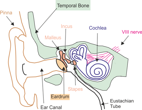
Figure 2.1
A
cross-section of the side of the head, showing structures of the outer, middle,
and inner ear.
From an acoustical point of view,
the fluids inside the cochlea are essentially (slightly salted) water, and we had already mentioned earlier (section 1.7),
that the acoustic impedance of water is much higher than that of air. This
means, simply put, that water must be pushed much harder than air if the water
particles are to oscillate with the same velocity. Consequently, a sound wave
traveling through air and arriving at a water surface,
cannot travel easily across the air-water boundary. The air-propagated sound
pressure wave is simply too weak to impart similar size vibrations onto the
water particles, and most of the vibration will therefore fail to penetrate
into the water and will be reflected back at the boundary. To achieve an
efficient transmission of sound from the air-filled ear canal to the fluid-filled
cochlea, it is therefore necessary to concentrate the pressure of the sound
wave onto a small spot, and that is precisely the purpose of the middle ear.
The middle ear collects the sound pressure over the relatively large area of
the eardrum (a surface area of about 500 mm2) and focuses it on the
much smaller surface area of the stapes footplate, which is about twenty times
smaller. The middle ear thus works a little bit like a thumb tack, collecting
pressure over a large area on the blunt, thumb end, and concentrating it on the
sharp end, allowing it to be pushed through into a material that offers a high
mechanical resistance.
Of course, a thumb tack is usually
made of just one piece, but the middle ear contains three bones, which seems
more complex than it needs to be to simply concentrate forces. The middle ear
is mechanically more complex in part because this complexity allows for the
mechanical coupling the middle ear provides to be regulated. For example, a
tiny muscle called the stapedius spans the space between
the stapes and the wall of the inner ear, and if this muscle is contracted, it reduces
the motion of the stapes, apparently to protect the delicate inner ear
structures from damage due to very loud sounds.
Sadly, the stapedius
muscle is not under our conscious control, but is contracted through an
unconscious reflex when we are exposed to continuous loud sounds. And because
this stapedius reflex, sometimes called the acoustic
reflex, is relatively slow (certainly compared to the speed of sound), it
cannot protect us from very sudden loud, explosive noises like gunfire. Such
sudden, very intense sounds are therefore particularly likely to damage our
hearing. The stapedius reflex is, however, also
engaged when we vocalize ourselves, so if you happen to be a gunner, talking or
singing to yourself aloud while you prepare to fire might actually help protect
your hearing.2 The stapedius
reflex also tends to affect some frequencies more than others, and the fact
that it is automatically engaged each time we speak may help explain why most
people find their own recorded voice sounds somewhat strange and unfamiliar.
But even with the stapedius muscle relaxed, the middle ear cannot transmit
all sound frequencies to the cochlea with equal efficiency. The middle ear ossicles themselves, although small and light, nevertheless
have some inertia that prevents them from transmitting very high frequencies.
Also, the ear canal, acting a bit like an organ pipe, has its own resonance
property. The shape of the human audiogram, the function that describes how our
auditory sensitivity varies with sound frequency described in section 1.8, is
thought to reflect mostly mechanical limitations of the outer and middle ear.
Animals with good hearing in the
ultrasonic range, like mice or bats, tend to have particularly small, light
middle ear ossicles. Interesting exceptions to this
are dolphins and porpoises, animals with an exceptionally wide frequency range,
from about 90 Hz up to 150 kHz or higher. Dolphins therefore can hear
frequencies three to four octaves higher than those audible to man. But, then,
dolphins do not have an impedance matching problem that needs to be solved by
the middle ear. Most of the sounds that dolphins listen to are already
propagating through the high-acoustic-impedance environment of the ocean, and,
as far as we know, dolphins collect these waterborne sounds not through their
ear canals (which, in any event, are completely blocked off by fibrous tissue),
but through their lower jaws, from where they are transmitted through the
temporal bone to the inner ear.
But for animals adapted to life on
dry land, the role of the middle ear is clearly an important one. Without it,
most of the sound energy would never make it into the inner ear. Unfortunately,
the middle ear, being a warm and sheltered space, is also a cozy environment
for bacteria, and it is not uncommon for the middle ear to harbor infections.
In reaction to such infections, the blood vessels of the lining of the middle
ear will become porous, allowing immune cells
traveling in the bloodstream to penetrate into the middle ear to fight the
infection, but along with these white blood cells there will also be fluid
seeping out of the bloodstream into the middle ear space. Not only do these
infections tend to be quite painful, but also, once the middle ear cavity fills
up with fluid, it can no longer perform its purpose of providing an impedance
bridge between the air-filled ear canal and the fluid-filled cochlea. This
condition, known as otitis media with effusion, or, more commonly, as glue ear, is one of the most
common causes of conductive hearing loss.
Thankfully, it is normally fairly
short lived. In most cases, the body’s immune system (often aided by antibiotics)
overcomes the infection, the middle ear space clears
within a couple of weeks, and normal hearing sensitivity returns. A small duct,
known as the Eustachian tube, which connects the middle ear to the back of the
throat, is meant to keep the middle ear drained and ventilated and therefore
less likely to harbor bacteria. Glue ear tends to be more common in small
children because the Eustachian tube is less efficient at providing drainage in
their smaller heads. Children who suffer particularly frequent episodes of otitis media can often benefit from the surgical
implantation of a grommet, a tiny piece of plastic tubing, into the eardrum to
provide additional ventilation.
When the middle ear operates as it
should, it ensures that sound waves are efficiently transmitted from the eardrum
through the ossicles to the fluid-filled interior of
the cochlea. Figure 2.2 shows the structure of the
cochlea in a highly schematic, simplified drawing that is and not to scale. For
starters, the cochlea in mammals is a coiled structure (see figure
2.1), which takes two and a half turns in the human, but
in figure 2.2,
it is shown as if it was unrolled into a straight tube. The outer wall of the
cochlea consists of solid bone, with a membrane lining. The only openings in
the hard bony shell of the cochlea are the oval
window, right under the stapes footplate, and the round window, which is situated below. As the stapes vibrates to
and fro to the rhythm of the sound, it pushes and pulls on the delicate
membrane covering the oval window.
Every time the stapes pushes
against the oval window, it increases the pressure in the fluid-filled spaces
of the cochlea. Sound travels very fast in water, and the cochlea is a small
structure, so we can think of this pressure increase as occurring almost
instantaneously and simultaneously throughout the entire cochlea. But because
the cochlear fluids are incompressible and almost entirely surrounded by a hard
bony shell, these forces cannot create any motion inside the cochlea unless the
membrane covering the round window bulges out a little every time the oval
window is pushed in, and vice versa. In principle, this can easily happen.
Pressure against the oval window can cause motion of a fluid column in the
cochlea, which in turn causes motion of the round window.
However, through almost the entire
length of the cochlea runs a structure known as the basilar membrane, which subdivides the fluid-filled spaces inside
the cochlea into upper compartments (the scala vestibuli and scala media) and lower
compartments (the scala tympani). We refer to them as
upper and lower here because they are usually drawn that way, and we will stick
to this convention in our drawings; but bear in mind that, because the cochlea
is actually a coiled structure, whether the scala
tympani is below or above the scala vestibuli depends on where we look along the cochlear coil.
The scala tympani is below the scala
vestibuli for the first, third, and fifth half turn,
but above for the second and fourth. (Compare figure 2.1.)
The basilar membrane has
interesting mechanical properties: It is narrow, thick, and stiff at the basal end of the cochlea (i.e., near
the oval and round windows), but wide and thick and floppy at the far, apical end. In the human, the distance
from the stiff basal to the floppy apical end is about 3.5 cm. A sound wave
that wants to travel from the oval window to the round window therefore has
some choices to make: It could take a short route (labeled A in figure
2.2), which involves traveling through only small amounts
of fluid, but pushing through the stiffest part of the basilar membrane, or it
could take a long route (B), traveling through more fluid, to reach a part of
the basilar membrane that is less stiff. Or, indeed, it could even travel all
the way to the apex, the so-called helicotrema, where
the basilar membrane ends and the scala vestibuli and scala tympani are
joined. There, the vibration would have to travel through no membrane at all. And
then there are all sorts of intermediate paths, and you might even think that,
if this vibration really travels sound wave style, it should not pick any one
of these possible paths, but really travel down all of them at once.
In principle, that is correct, but
just as electrical currents tend to flow to a proportionally greater extent
down paths of smaller resistance, most of the mechanical energy of the sound
wave will travel through the cochlea along the path that offers the smallest
mechanical resistance. If the only mechanical resistance was that offered by
the basilar membrane, the choice would be an easy one: All of the mechanical
energy should travel to the apical end, where the stiffness of the basilar
membrane is low. And low-frequency sounds do indeed predominantly choose this long
route. However, high-frequency sounds tend not to, because at high frequencies
the long fluid column involved in a path via the apex itself
is becoming a source of mechanical resistance, only that this resistance is due
to inertia rather than stiffness.
Figure 2.2
Schematic drawing
showing the cochlea unrolled, in cross-section. The gray shading represents the
inertial gradient of the perilymph and the stiffness
gradient of the basilar membrane.
Imagine a sound wave trying to
push the oval window in and out, very rapidly, possibly several thousand times
a second for a high-frequency tone. As we have already discussed, the sound
wave will succeed in affecting the inside of the cochlea only if it can push in
and then suck back the cochlear fluids in the scala vestibuli, which in turn pushes and pulls on the basilar
membrane, which in turns pushes and pulls on the fluid in the scala tympani, which in turn pushes and pulls on the round
window. This chain of pushing and pulling motion might wish to choose a long
route to avoid the high mechanical resistance of the stiff basal end of the
basilar membrane, but the longer route will also mean that a greater amount of
cochlear fluid, a longer fluid column, will first have to be accelerated and
then slowed down again, twice, on every push and pull cycle of the vibration.
Try a little thought experiment: Imagine
yourself taking a fluid-filled container and shaking it to and fro as quickly
as you can. First time round, let the fluid-filled container be a small perfume
bottle. Second time around, imagine it’s a barrel the size of a bathtub. Which
one will be easier to shake? Clearly, if you have to try to push and pull
heavy, inert fluids forward and backward very quickly, the amount of fluid
matters, and less is better. The inertia of the fluid poses a particularly
great problem if the vibration frequency is very high. If you want to generate
higher-frequency vibrations in a fluid column, then you will need to accelerate
the fluid column both harder and more often. A longer path, as in figure 2.2B,
therefore presents a greater inertial resistance to vibrations that wish to
travel through the cochlea, but unlike the stiffness resistance afforded by the
basilar membrane, the inertial resistance does not affect all frequencies to
the same extent. The higher the frequency, the greater the extra effort
involved in taking a longer route.
The cochlea is thus equipped with
two sources of mechanical resistance, one provided by the stiffness of the
basilar membrane, the other by inertia of the cochlear fluids, and both these
resistances are graded along the cochlea, but they run in opposite directions.
The stiffness gradient decreases as we move further away from the oval window,
but the inertial gradient increases. We have tried to illustrate these
gradients by gray shading in figure
2.2.
Faced with these two sources of
resistance, a vibration traveling through the cochlea will search for a
“compromise path,” one which is long enough that the stiffness has already
decreased somewhat, but not so long that the inertial resistance has already
grown dramatically. And because the inertial resistance is frequency dependent,
the optimal compromise, the path of
overall lowest resistance, depends on the frequency. It is long for low
frequencies, which are less affected by inertia, and increasingly shorter for
higher frequencies. Thus, if we set the stapes to vibrate at low
frequencies, say a few hundred Hertz, we will cause vibrations in the basilar
membrane mostly at the apex, a long way from the oval windows; but as we
increase the frequency, the place of maximal vibration on the basilar membrane
shifts toward the basal end. In this manner, each point of the basilar membrane
has its own “best frequency,” a frequency that will make this point on the
basilar membrane vibrate more than any other (see figure
2.3).
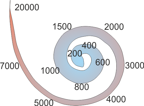
Figure 2.3
Approximate best
frequencies of various places along the basilar membrane, in hertz.
This property makes it possible
for the cochlea to operate as a kind of mechanical frequency analyzer. If it is
furnished with a sound of just a single frequency, then the place of maximal
vibration in the basilar membrane will give a good indication of what that
frequency is, and if we feed a complex tone containing several frequencies into
the cochlea, we expect to see several peaks of maximal excitation, one
corresponding to each frequency component in the input signal. (The book’s
website shows a little animation illustrating this <flag>). Because of
its ability to decompose the frequency content of vibrations arriving at the
oval window, the cochlea has sometimes been described as a biological Fourier
analyzer. Mathematically, any transformation that decomposes a waveform into a
number of components according to how well they match a set of sinusoidal basis
functions might be referred to as a Fourier method, and if we understand Fourier
methods in quite such broad terms, then the output of the cochlea is certainly
Fourier-like. However, most texts on engineering mathematics, and indeed our
discussions in chapter 1, tend to define Fourier transforms in quite narrow and
precise terms, and the operation of the cochlea, as well as its output, does
differ from that of these “standard Fourier transforms” in important ways,
which are worth mentioning.
Perhaps the most “standard” of all
Fourier methods is the so-called discrete Fourier transform (DFT), which
calculates amplitude and phase spectra by projecting input signals onto pure
sine waves, which are spaced linearly along the frequency axis. Thus, the DFT
calculates exactly one Fourier component for each harmonic of some suitably chosen
lowest fundamental frequency. A pure-tone frequency that happens to coincide
with one of these harmonics will excite just this one frequency component, and
the DFT can, in principle, provide an extremely sharp frequency resolution
(although in practice there are limitations, which we had described in section
1.4 under windowing). The cochlea really does nothing of the sort, and it is
perhaps more useful to think of the cochlea as a set of mechanical filters.
Each small piece of the basilar membrane, together with the fluid columns
linking it to the oval and round windows, forms a small mechanical filter
element, each with its own resonance frequency, which is determined mostly by
the membrane stiffness and the masses of the fluid columns. Unlike the
frequency components of a DFT, these cochlear filters are not spaced at linear
frequency intervals. Instead, their spacing is approximately logarithmic. Nor
is their frequency tuning terribly sharp, and their tuning bandwidth depends on
the best (center) frequency of each filter (the equivalent rectangular
bandwidth, or ERB, of filters in the human cochlea is, very roughly, 12% of the
center frequency, or about one-sixth of an octave, but it tends to be broader
for very low frequencies).
We have seen in section 1.5, if a
filter is linear, then all we need to know about it is its impulse response. As
we shall see in following sections, the mechanical filtering provided by the
cochlea is neither linear, nor is it time invariant. Nevertheless, a set of
linear filters can provide a useful first-order approximation of the mechanical
response of the basilar membrane to arbitrary sound inputs. A set of filters
commonly used for this purpose is the gamma-tone filter bank. We had already
encountered the gamma-tone filter in figure 1.13. Gamma-tone filters with
filter coefficients to match research on the human auditory system by
researchers like Roy Patterson and Brian Moore have been implemented in Matlab computer code by Malcolm Slaney; the code is freely
available and easy to find on the Internet. Figure 2.4
shows gamma-tone approximations to the impulse responses of fifteen sites
spaced regularly along the basilar membrane between the 400-Hz region near the apex to the 10-kHz region near the base,
based on Malcolm Slaney’s code. The filters are arranged by best frequency, and
the best frequencies of each of the filters are shown along the vertical (but
note that in this plot, the y-coordinate does indicate the amplitude of the
basilar membrane vibration, not the frequency).
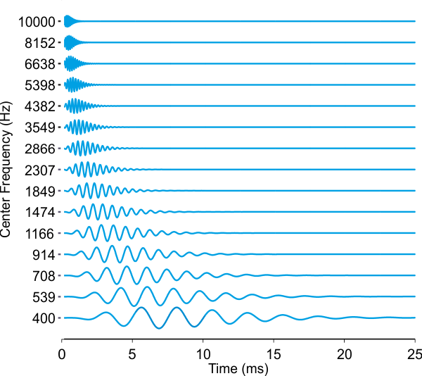
Figure 2.4
A gamma-tone filter
bank can serve as a simplified model of the basilar membrane.
One thing that is very obvious in
the basilar membrane impulse responses shown in figure 2.4
is that the high-frequency impulse responses are much faster than the low-frequency
ones, in the sense that they operate over a much shorter time window. If you
remember the discussion of the time windows in section 1.5, you may of course
appreciate that the length of the temporal analysis window that is required to
achieve a frequency resolution of about 12% of the center frequency can be
achieved with proportionally shorter time windows as the center frequency
increases, which explains why the impulse responses of basal, high-frequency
parts of the basilar membrane are shorter than those of the apical, low-frequency
parts. A frequency resolution of 12% of the center frequency does of course
mean that, in absolute terms, the high-frequency region of the basilar membrane
achieves only a poor spectral resolution, but a high-temporal resolution, while
for the low-frequency region the reverse is true.
One might wonder to what extent
this is an inevitable design constraint, or whether it is a feature of the
auditory system. Michael Lewicki (2002) has argued
that it may be a feature, that these basilar membrane filter shapes may in fact
have been optimized by evolution, that they form, in
effect, a sort of “optimal compromise” between frequency and time resolution
requirements to maximize the amount of information that the auditory system can
extract from the natural environment. The details of his argument are beyond
the scope of this book, and rather than examining the reasons behind the
cochlear filter shapes further, we shall look at their consequences in a little
more detail.
In section 1.5 we introduced the
notion that we can use the impulse responses of linear filters to predict the
response of these filters to arbitrary inputs, using a mathematical technique
called convolution. Let us use this technique and gamma-tone filter banks to
simulate the motion of the basilar membrane to a few sounds, starting with a
continuous pure tone.
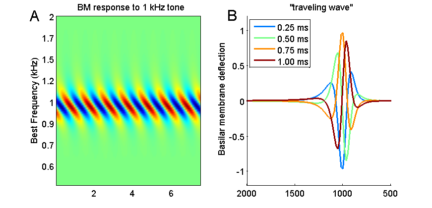
Figure 2.5
Basilar
membrane response to a pure tone. Systematic differences in amplitude and time
(phase) of the cochlear filters creates a traveling wave.
Figure 2.5A shows the simulated response of
a small piece of the basilar membrane near the 1-kHz region to a 1-kHz tone.
The best frequencies of the corresponding places on the basilar membrane are
plotted on the vertical, y-axis, the gray scale shows how far the basilar
membrane is deflected from its resting position, and the x-axis shows time. You
may recall from our section on filtering that linear filters cannot invent
frequencies: Given a sine wave input, they will produce a sine wave output, but
the sine wave output may be scaled and shifted in time. The simulated basilar
membrane filters behave in just that way too: Each point on the basilar
membrane (each row in the top panel of figure 2.5)
oscillates at 1 kHz, the input frequency, but those points with best
frequencies closest to the input frequency vibrate most strongly, and those
with best frequencies a far removed from the input frequency vibrate hardly at
all. That much you would probably have expected.
But you may also note that the
vibrations of the parts of the basilar membrane tuned to frequencies below 1
kHz appear time shifted or delayed relative to those tuned above 1 kHz. This
comes about because the mechanical filters that make up the basilar membrane
are not all in phase with each other (if you look at figure
2.4, you will see that the impulse
responses of the lower-frequency filters rise to their first peak later than those
of the high-frequency ones), and this causes the response of the lower-frequency
filters to be slightly delayed relative to the earlier ones.
Due to this slight time shift, if
you were to look down on the basilar membrane, you would see a traveling wave, that
is, it would look as if the peak of the oscillation starts out small at the
basal end, grows to reach a maximum at the best
frequency region, and then shrinks again. This traveling wave is shown
schematically in figure 2.5B.
This panel shows snapshots of the basilar membrane deflection (i.e., vertical
cuts through figure 2.5A)
taken at 0.25-ms intervals, and you can see that the earliest (black) curve has
a small peak at roughly the 1.1-kHz point, which is followed 0.25 ms later by a
somewhat larger peak at about the 1.05-kHz point (dark gray curve), then a high
peak at the 1-kHz point (mid gray), and so on. The peak appears to travel.
The convention (which we did not
have the courage to break with) seems to be that every introduction to hearing
must mention this traveling wave phenomenon, even though it often creates more
confusion than insight among students. Some introductory texts describe the
traveling wave as a manifestation of sound energy as it travels along the
basilar membrane, but that can be misleading, or at least, it does not necessarily
clarify matters. Of course would could imagine that a
piece of basilar membrane, having been deflected from its neutral resting
position, would, due to its elasticity, push back on the fluid, and in this
manner it may help “push it along”. And the basilar membrane is continuous, it
is not a series of disconnected strings or fibers, so if one patch of the
basilar membrane is being pushed up by the fluid below it, it will pull gently
on the next patch along to which it is attached. Nevertheless, the contribution
that the membrane itself makes to the propagation of mechanical energy through the cochlea
is likely to be small, so it is probably most accurate to imagine the
mechanical vibrations as travelling “along” the membrane only in the sense that
they travel mostly through the fluid next
to, the membrane, and then pass
through the basilar membrane as they near the point of lowest resistance,
as we have tried to convey in figure 2.2.
The traveling wave may then be mostly a curious side effect of the fact that
the mechanical filters created by each small piece of basilar membrane,
together with the associated cochlear fluid columns, all happen to be slightly
out of phase with each other. Now, the last few sentences contained a lot of “perhaps”
and “maybe”, and you may well wonder, if the travelling wave is considered such
an important phenomenon, why is there not more clarity and certainty? But bear
in mind that the cochlea is a tiny, delicate structure buried deep in the
temporal bone (which happens to be the hardest bone in your body), which makes
it very difficult to take precise and detailed measurements of almost any
aspect of the operation of the cochlea.
Perhaps the traveling wave gets so much
attention because experimental observations of traveling waves on the surface
of the basilar membrane, carried out by Georg von Bekesy in the 1950s, were
among the earliest, and hence most influential, studies into the physiology of
hearing, and they won him the Nobel Prize in 1961. They were also useful
observations. If the basilar membrane exhibited standing waves, rather than
traveling ones, it would indicate that significant amounts of sound energy
bounce back from the cochlear apex, and the picture shown in figure
2.2 would need to be revised. The observation of
traveling, as opposed to standing, waves therefore provides useful clues as to
what sort of mechanical processes can or cannot occur within the cochlea.
But while the traveling wave
phenomenon can easily confuse, and its importance may sometimes be overstated,
the related notion of cochlear place
coding for frequency, or tonotopy,
is undoubtedly an important one. Different frequencies will create maximal
vibrations at different points along the basilar membrane, and a mechanism that
could measure the maxima in the vibration amplitudes along the length of the
cochlea could derive much useful information about the frequency composition of
the sound. The basilar membrane is indeed equipped with such a mechanism; it is
known as the organ of Corti, and we shall describe
its function shortly. But before we do, we should also point out some of the
implications and limitations of the mechanical frequency-filtering process of
the cochlea.
One very widespread misconception
is that there is a direct and causal relationship between cochlear place code
and the perception of musical pitch (tone height); that is, if I listen to two
pure tones in succession—say first a 1,500-Hz and then a 300-Hz tone—the 300-Hz
tone will sound lower because it
caused maximal vibration at a point further away from the stapes than the 1,500-Hz
one did. After our discussion of sound production in chapter 1, you probably
appreciate that most sounds, including most “musical” ones with a clear pitch,
contain numerous frequency components and will therefore lead to significant
vibration on many places along the basilar membrane at once, and trying to
deduce the pitch of a sound from where on the basilar membrane vibration
amplitudes are maximal is often impossible. In fact, many researchers currently
believe that the brain may not even try to determine the pitch of real, complex
sounds that way (an animation on the book’s web page showing the response of
the basilar membrane to a periodic click train illustrates this <flag>).
We will look at pitch perception
in much greater detail in chapter 3, but to convey a flavor of some of the
issues, and give the reader a better feeling of the sort of raw material the
mechanical filtering in the cochlea provides to the brain, we shall turn once
more to a gamma-tone filter bank to model basilar membrane vibrations—this time
not in response to the perhaps banal 1-kHz pure tone we examined in figure
2.5, but instead to the sound of a spoken word. Figure 2.6 compares the basilar
membrane response and the spectrogram of the spoken word “head,” which we had
already encountered in figure 1.16. You may recall, from section 1.6 in chapter
1, that this spoken word contains a vowel /ae/,
effectively a complex tone created by the glottal pulse train, which generates
countless harmonics, and that this vowel occurs between two broadband
consonants, a fricative /h/ and a plosive /d/. The spacing of the harmonics in
the vowel will determine the perceived pitch (or “tone height”) of the word. A
faster glottal pulse train means more widely spaced harmonics, and hence a
higher pitch.
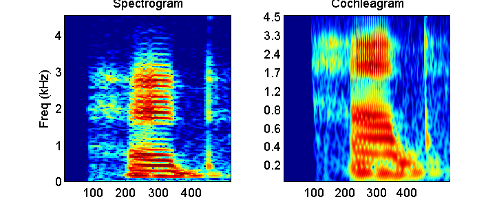
Figure 2.6
Spectrogram
of, and basilar membrane response to, the spoken word “head” (compare figure
1.16).
If we make a spectrogram of this
vowel using relatively long analysis time windows to achieve high spectral
resolution, then the harmonics become clearly visible as stripes placed at
regular frequency intervals (left panel of figure 2.6).
If we pass the sound instead through a gamma-tone cochlear filter model, many
of the higher harmonics largely disappear. The right panel of figure
2.6 illustrates this. Unlike in figure 2.5, which shows
basilar membrane displacement at a very fine time resolution, the time
resolution here is coarser, and the grayscale shows the logarithm of the RMS
amplitude of the basilar membrane movement at sites with best frequencies, as
shown on the y-axis. (We plot the log of the RMS amplitude to make the output
as comparable as possible to the spectrogram, which, by convention, plots
relative sound level in dB; that is, it also uses a logarithmic scale). As we already
mentioned, the best frequencies of cochlear filters are not spaced linearly
along the basilar membrane. (Note that the frequency axes for the two panels in
figure 2.6 differ.)
A consequence of this is that the
cochlear filters effectively resolve, or zoom in to the lowest frequencies of
the sound, up to about 1 kHz or so, in considerable detail. But in absolute
terms, the filters become much less sharp for higher frequencies, so that at
frequencies above 1 kHz individual harmonics are no longer apparent. Even at
only moderately high frequencies, the tonotopic place
code set up by mechanical filtering in the cochlea thus appears to be too crude
to resolve the spectral fine structure necessary to make out higher harmonics3.
The formant frequencies of the speech sound, however, are still readily
apparent in the cochlear place code, and the temporal onsets of the consonants
/h/ and /t/ also appear sharper in the cochleagram
than in the long time window spectrogram shown on the left. In this manner, a cochleagram may highlight different features of a sound from
a standard spectrogram with a linear frequency axis and a fixed spectral
resolution.
2.2 Hair Cells, Transduction from Vibration to Voltage
As we have seen, the
basilar membrane acts as a mechanical filter bank that separates out different
frequency components of the incoming sound. The next stage in the auditory
process is the conversion of the mechanical vibration of the basilar membrane
into a pattern of electrical excitation that can be encoded by sensory neurons
in the spiral ganglion of the inner ear for transmission to the brain. As we mentioned
earlier, the site where this transduction from mechanical to electrical signals
takes place is the organ of Corti, a delicate
structure attached to the basilar membrane, as shown in figure
2.7.
Figure 2.7 shows only a schematic drawing of
a slice through the cochlea, and it is important to appreciate that the organ
of Corti runs along the entire length of the basilar
membrane. When parts of the basilar membrane vibrate in response to acoustic
stimulation, the corresponding parts of the organ of Corti
will move up and down together with the membrane. As the inset in figure
2.7 shows, the organ of Corti
has a curious, folded structure. In the foot of the structure, the portion that
sits directly on the basilar membrane, one finds rows of sensory hair cells. On
the modiolar side (the side closer to the modiolus, i.e., the center of the cochlear spiral), the
organ of Corti curves up and folds back over to form
a little “roof,” known as the “tectorial membrane,”
which comes into close contact with the stereocilia
(the hairs) on the sensory hair cells. It is thought that, when the organ of Corti vibrates up and down, the tectorial
membrane slides over the top of the hair cells, pushing the stereocilia
toward the modiolar side as the organ of Corti is pushed up, and in the opposite direction when it
is pushed down.
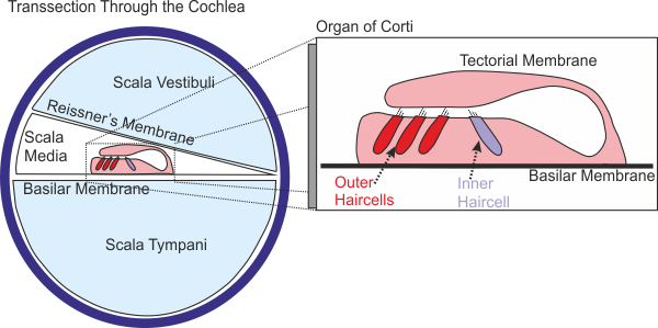
Figure 2.7
Cross-section
of the cochlea, and schematic view of the organ of Corti.
You may have noticed that the
sensory hair cells come in two flavors: inner hair cells and outer hair cells.
The inner hair cells form just a single row of cells all along the basilar
membrane, and they owe their name to the fact that they sit closer to the modiolus, the center of the cochlea, than the outer hair
cells. Outer hair cells are more numerous, and typically form between three and
five rows of cells. The stereocilia of the outer hair
cells may actually be attached to the tectorial
membrane, while those of the inner hair cells may be driven mostly by fluid
flowing back and forth between the tectorial membrane
and the organ of Corti; however, both types of cells
experience deflections of their stereocilia, which
reflect the rhythm and the amplitude of the movement of the basilar membrane on
which they sit.
Also, you may notice in figure
2.7 that the cochlear compartment above the basilar
membrane is divided into two subcompartments, the scala media and the scala vestibuli, by a membrane known as Reissner’s
membrane. Unlike the basilar membrane, which forms an important and
systematically varying mechanical resistance that we discussed earlier, Reissner’s membrane is very thin and is not thought to
influence the mechanical properties of the cochlea in any significant way. But,
although Reissner’s membrane poses no obstacle to
mechanical vibrations, it does form an effective barrier to the movement of
ions between the scala media and the scala vestibuli.
Running along
the outermost wall of the scala media, a structure
known as the stria vascularis
leaks potassium (K+) ions from the bloodstream into the scala media. As the K+ is trapped in the scala media by Reissner’s
membrane above and the upper lining of the basilar membrane below, the K+
concentration in the fluid that fills the scala
media, the endolymph, is much higher than that in the
perilymph, the fluid that fills the scala vestibuli and the scala tympani. The stria vascularis also sets up an electrical voltage gradient,
known as the endocochlear potential, across the
basilar membrane. These ion concentration and voltage gradients provide the driving
force behind the transduction of mechanical to electrical signals in the inner
ear. Healthy inner ears have an endocochlear
potential of about 80 to100 mV.
The stereocilia
that stick out of the top of the hair cells are therefore bathed in an
electrically charged fluid of a high K+ concentration, and a wealth
of experimental evidence now indicates that the voltage gradient will drive K+
ions into the hair cells through the stereocilia, but
only if the stereocilia are deflected. Each hair cell
possesses a bundle of several dozen stereocilia, but
the stereocilia in the bundle are not all of the same
length. Furthermore, the tips of the stereocilia in
each bundle are connected by fine protein fiber strands known as “tip links.”
Pushing the hair cell bundle toward the longest stereocilium
will cause tension on the tip links, while pushing the bundle in the other
direction will release this tension. The tip links are thought to be connected
to stretch receptors, tiny ion channels that open in response to stretch on the
tip links, allowing K+ ions to flow down the electrical and concentration
gradient from the perilymph into the hair cell This
is illustrated schematically in figure 2.8.
Since K+ ions carry positive charge, the K+ influx is
equivalent to an inward, depolarizing current entering the hair cell.
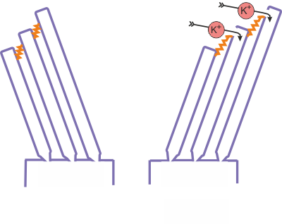
Figure 2.8
Schematic
of the hair cell transduction mechanism.
Thus, each cycle of the vibration
of the basilar membrane causes a corresponding cycle of increasing and
decreasing tension on the tip links. Because a greater tension on the tip links
will pull open a greater number of K+ channels, and because the K+
current thereby allowed into the cell is proportional to the number of open
receptors, the pattern of mechanical vibration is thus translated into an
analogous pattern of depolarizing current. The larger the
deflection of the cilia, the greater the current. And the amount of
depolarizing current in turn is manifest in the hair cell’s membrane potential.
We therefore expect the voltage across the hair cell’s membrane to increase and
decrease periodically in synchrony with the basilar membrane vibration.
Recordings made from individual
hair cells have confirmed that this is indeed the case, but they also reveal
some perhaps unexpected features. Hair cells are tiny, incredibly delicate
structures, typically only somewhere between 15 and 70 µm tall (Ashmore, 2008), with their stereocilia
protruding for about 20 μm at most. Gifted
experimenters have nevertheless been able to poke intracellular recording
electrodes into living hair cells from inside the cochlea of experimental
animals (mostly guinea pigs or chickens), to record their membrane voltage in
response to sounds. Results from such recording experiments are shown in figure
2.9.
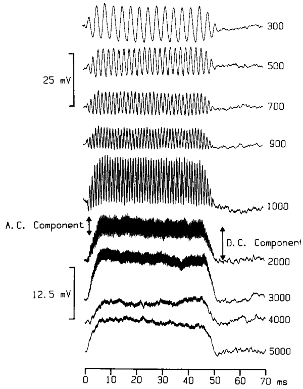
Figure 2.9
Changes
in hair cell membrane voltage in response to sinusoidal stimulation of the stereocilia.
From figure 9 of
Palmer and Russell (1986), Hear Res 24:1-15, with permission from Elsevier.
The traces show changes in the
measured membrane potential in response to short bursts of sinusoidal vibration
of the hair cell bundle, with frequencies shown to the right. At low vibration
frequencies, the membrane potential behaves very much as we would expect on the
basis of what we have learned so far. Each cycle of the mechanical stimulation
is faithfully reflected in a sinusoidal change in the membrane voltage.
However, as the vibration frequency increases into the kilohertz range,
individual cycles of the vibration become increasingly less visible in the
voltage response, and instead the cell seems to undergo a continuous
depolarization that lasts as long as the stimulus.
The cell membrane acts much like a
small capacitor, which needs to be discharged every time a deflection of the
hair cell bundle is to be reflected in the membrane voltage. This discharging,
and subsequent recharging, of the cell membrane’s capacitance cannot occur
quickly. When the stimulation frequency increases from a few hundred to a few
thousand Hertz, therefore, the hair cell gradually changes from an AC (alternating
current) mode, where every vibration cycle is represented, to a DC (direct
current) mode, in which there is a continuous depolarization, whose magnitude
reflects the amplitude of the vibration. The DC mode
comes about through a slight asymmetry in the effects of the stretch receptor
currents. Opening the stretch receptors can depolarize a hair cell more than
closing the channels hyperpolarizes it. The loss of AC at high frequencies has
important consequences for the amount of detail that the ear can capture about
the temporal fine structure of a sound, as we shall see in greater detail in
section 2.4.
So far, we have discussed hair
cell function as if hair cells are all the same, but you already know that
there are outer and inner cells, and that some of live
on high-frequency parts of the basilar membrane and others on low-frequency
parts. Do they all function in the same way, or are there differences one ought
to be aware of? Let us first consider high- versus low-frequency parts. If you
consider the electrical responses shown in figure 2.9
with the tonotopy plot we have seen in figure 2.3,
then you may realize that in real life most hair cells rarely find the need to
switch from AC to DC mode. Hair cells on the basal-most part of the cochlea
will, due to the mechanical filtering of the cochlea, experience only
high-frequency sounds and should therefore only operate in AC mode.
Well, that is sort of true, but
bear in mind that, in nature, high-frequency sounds are rarely continuous, but
instead fluctuate over time. A hair cell in the 10-kHz region of the cochlea
will be able to encode such amplitude modulations in its membrane potential,
but again only to frequencies up to a few kilohertz at most, for the same
reasons that a hair cell in the low-frequency regions in the cochlea can follow
individual cycles of the sound wave only up to a few kilohertz. Nevertheless,
you might wonder whether the hair cells in the high- or low-frequency regions
do not exhibit some type of electrical specialization that might make them
particularly suitable to operate effectively at their own best frequency.
Hair cells from the inner ear of
reptiles and amphibians, indeed, seem to exhibit a degree of electrical tuning that
makes them particularly sensitive to certain frequencies (Fettiplace
& Fuchs, 1999). But the inner ears of these lower vertebrates are
mechanically much more primitive than those of mammals, and so far, no evidence
for electrical tuning has been found in mammalian hair cells. Present evidence
suggests that the tuning of mammalian hair cells is therefore predominantly or
entirely a reflection of the mechanics of the piece of basilar membrane on
which they live (Cody & Russell, 1987). But what about
differences between outer and inner hair cells? These turn out to be
major, and important—so much so that they deserve a separate subsection.
2.3 Outer Hair Cells and Active Amplification
At parties, there are
sometimes two types of people: those who enjoy listening to conversation, and
those who prefer to dance. With hair cells, it is similar. The job of inner
hair cells seems to be to talk to other nerve cells, while that of outer hair
cells is to dance. And we don’t mean dance in some abstract or figurative
sense, but quite literally, in the sense of “moving in tune to the rhythm of
the music.” In fact, you can find a movie clip showing a dancing hair cell on
the Internet. This movie was made in the laboratory of Prof. Jonathan Ashmore, He and his colleagues isolated individual outer
hair cells from the cochlea of a guinea pig, fixed it to a patch pipette, and
through that patch pipette injected an electrical current waveform of the song “Rock
Around the Clock.” Under the microscope, one can clearly see that the outer
hair cell responds to this electrical stimulation by stretching and contracting
rhythmically, following along to the music.
Outer hair cells (OHCs) possess a unique, only recently characterized motor
protein in their cell membranes, which causes them to contract every time they
are depolarized. This protein, which has been called “prestin,”
is not present in inner hair cells or any other cells of the cochlea. The name prestin is very apt. It has the same root as the Italian presto for “quick,” and prestin is one of the fastest biological motors known to
man—much, much faster than, for example, the myosin molecules responsible for
the contraction of your muscles. Prestin will not
cause the outer hair cells to move an awful lot; in fact, they appear to
contract by no more than about 4% at most. But it appears to enable them to
carry out these small movements with astounding speed. These small but
extremely fast movements do become rather difficult to observe. Most standard
video cameras are set up to shoot no more than a few dozen frames a second
(they need to be no faster, given that the photoreceptors in the human eye are
comparatively slow).
To measure the physiological speed
limit of the outer hair cell’s prestin motor,
therefore, requires sophisticated equipment, and even delivering very fast
signals to the OHCs to direct them to move as fast as
they can is no easy matter (Ashmore, 2008). Due to
these technological difficulties, there is still some uncertainty about exactly
how fast OHCs can move, but we are quite certain they
are at least blisteringly, perhaps even stupefyingly
fast, as they have been observed to undergo over 70,000 contraction and
elongation cycles a second, and some suspect that the OHCs
of certain species of bat or dolphin, which can hear sounds of over 100 kHz,
may be able to move faster still.
The OHCs
appear to use these small but very fast movements to provide a mechanical
amplification of the vibrations produced by the incoming sound. Thus, it is
thought that, on each cycle of the sound-induced basilar membrane vibration,
the OHC’s stereocilia are
deflected, which causes their membrane to polarize a little, which causes the
cells to contract, which somehow makes the basilar membrane move a little more,
which causes their stereocilia to be deflected a
little more, creating stronger depolarizing currents and further OHC
contraction, and so forth, in a feedforward spiral
capable of adding fairly substantial amounts of mechanical energy to otherwise
very weak vibrations of the basilar membrane. It must be said, however, that how
this is supposed to occur remains rather hazy.
What, for example, stops this
mechanical feedback loop from running out of control? And how exactly does the
contraction of the hair cells amplify the motion of the basilar membrane? Some
experiments suggest that the OHC contractions may cause them to “flick” their
hair cell bundles (Jia & He, 2005), and thereby pull
against the tectorial membrane (Kennedy, Crawford,
& Fettiplace, 2005), but this is not the only
possibility. They could also push sidewise, given that they do get fatter as
they contract. Bear in mind that the amplitude of the movement of OHCs is no more than a few microns at most, and they do
this work while imbedded in an extremely delicate structure buried deep inside
the temporal bone, and you get a sense of how difficult it is to obtain
detailed observations of OHCs in action in their
natural habitat. It is, therefore, perhaps more surprising how much we already
know about the function of the organ of Corti, than
that some details still elude us.
One of the things we know with
certainty is that OHCs are easily damaged, and animals
or people who suffer extensive and permanent damage to these cells are
subsequently severely or profoundly hearing impaired, so their role must be
critical. And their role is one of mechanical amplification, as was clearly
shown in experiments that have measured basilar membrane motion in living cochleas with the OHCs intact and
after they were killed off.
These experiments revealed a number
of surprising details. Figure 2.10,
taken from a paper by Ruggero et al. (1997), plots
the mechanical gain of the basilar membrane motion, measured in the cochlea of
a chinchilla, in response to pure tones presented at various frequencies and
sound levels. The gain is given in units of membrane velocity (mm/s) per unit
sound pressure (Pa). Bear in mind that the RMS velocity of the basilar membrane
motion must be proportional to its RMS amplitude (if the basilar membrane travels
twice as fast, it will have traveled twice as far), so the figure would look
much the same if it were plotted in units of amplitude per pressure. We can
think of the gain plotted here as the basilar membrane’s
“exchange rate,” as we convert sound pressure into basilar membrane vibration.
These gains were measured at the 9-kHz characteristic frequency (CF) point of
the basilar membrane, that is, the point which needs the lowest sound levels of
a 9-kHz pure tone to produce just measurable vibrations. The curves show the
gain obtained for pure-tone frequencies shown on the x-axis, at various sound
levels, indicated to the right of each curve. If this point on the basilar
membrane behaved entirely like a linear filter, we might think of its CF as a
sort of center frequency of its tuning curve, and would expect gains to drop
off on either side of this center frequency.
At low sound levels (5 or 10 dB),
this seems to hold, but as the sound level increases, the best frequency (i.e.,
that which has the largest gains and therefore the strongest response)
gradually shifts toward lower frequencies. By the time the sound level reaches
80 dB, the 9-kHz CF point on the basilar membrane actually responds best to
frequencies closer to 7 kHz. That is a substantial reduction in preferred
frequency, by almost 22%, about a quarter of an octave, and totally unheard of
in linear filters. If the cochlea’s tonotopy was responsible for our perception
of tone height in a direct and straightforward manner, then a piece of music
should rise substantially in pitch if we turn up the volume. That is clearly
not the case. Careful psychoacoustical studies have
shown that there are upward pitch shifts with increasing sound intensity, but
they are much smaller than a naïve cochlear place coding hypothesis would lead
us to expect given the nonlinear basilar membrane responses.

Figure 2.10
Gain of the basal
membrane motion, measured along various points on the basilar membrane (their
characteristic frequency is shown on the x-axis) in response to a 9-kHz tone
delivered at various sound levels (indicated by numbers to the right of each
curve).
From figure 10 of Ruggero
et al. (1997), J Acoust Soc Am 101:2151-2163., with permission from the Acoustical Society of
Another striking feature of figure
2.10 is that the gains, the exchange rates applied as we
can convert sound pressure to basilar membrane vibration, is not the same for
weak sounds as for intense sounds. The maximal gain for the weakest sounds
tested (5 dB SPL) is substantially greater than that obtained at the loudest
sounds tested (80 dB SPL). Thus, the OHC amplifier amplifies weaker sounds more
strongly than louder sounds, but the amplitude of basilar membrane vibrations
nevertheless still increases monotonically with sound level. In a way, this is very
sensible. Loud sounds are sufficiently intense to be detectable in any event,
only the weak sounds need boosting. Mathematically, an operation that amplifies
small values a lot but large values only a little bit is called a “compressive
nonlinearity.” A wide range of inputs (sound pressure amplitudes) is mapped (compressed)
onto a more limited range of outputs (basilar membrane vibration amplitudes).
The OHC amplifier in the inner ear
certainly exhibits such a compressive nonlinearity, and thereby helps make the millionfold range of amplitudes that the ear may be
experiencing in a day, and which we have described in section 1.8, a little
more manageable. This compressive nonlinearity also goes hand in hand with a
gain of up to about 60 dB for the weakest audible sounds (you may remember from
section 1.8 that this corresponds to approximately a thousandfold
increase of the mechanical energy supplied by the sound. This powerful, and nonlinear amplification of the sound wave by
the OHCs is clearly important—we would be almost
completely deaf without it, but from a signal processing point of view it is a
little awkward.
Much of what we learned about
filters in section 1.5, and what we used to model cochlear responses in section
2.1, was predicated on an assumption of linearity, where linearity, you may
recall, implies that a linear filter is allowed to change a signal only by
applying constant scale factors and
shifts in time. However, the action of OHCs means
that the scale factors are not
constant: They are larger for small-amplitude vibrations than for large ones.
This means that the simulations we have shown in figures 2.4 and 2.5 are,
strictly speaking, wrong. But were they only slightly wrong, but nevertheless useful
approximations that differ from the real thing in only small, mostly
unimportant details? Or are they quite badly wrong?
The honest answer is that, (a) it
depends, and (b) we don’t really know. It depends, because the cochlear nonlinearity,
like many nonlinear functions, can be quite well approximated by a straight
line as long as the range over which one uses this linear approximation remains
sufficiently small. So, if you try, for example, to model only responses to
fairly quiet sounds (say less than 40 dB), then your approximation will be much
better than if you want to model responses over an 80- or 90-dB range. And we
don’t really know because experimental data are limited, so that we do not have
a very detailed picture of how the basilar membrane really responds to complex
sounds at various sound levels. What we do know with certainty, however, is
that the outer hair cell amplifier makes responses of the cochlea a great deal
more complicated.
For example, the nonlinearity of
the outer hair cell amplifier may introduce frequency components into the
basilar membrane response that were not there in the first place. Thus, if you
stimulate the cochlea with two simultaneously presented pure tones, the cochlea
may in fact produce additional frequencies, known as distortion products (Kemp,
2002). In addition to stimulating inner hair cells, just like any externally
produced vibration would, these internally created frequencies may travel back
out of the cochlea through the middle ear ossicles to
the eardrum, so that they can be recorded with a microphone positioned in or
near the ear canal. If the pure tones are of frequencies f1 and f2,
then distortion products are normally observed at frequencies f1 + N(f2 -
f1), where N can be
any positive of negative whole number.
These so-called distortion product
otoacoustic emissions (DPOAEs)
provide a useful diagnostic tool, because they occur only when the OHCs are healthy and working as they should. And since, as
we have already mentioned, damage to the OHCs is by
far the most common cause of hearing problems, otoacoustic
emission measurements are increasingly done routinely in newborns or prelingual children in order to identify potential problems
early. (Alternatively to DPOAE measurements based on two tones presented at any
one time, clinical tests may use very brief clicks to look for transient evoked
otoacoustic emissions, or TEOAEs.
Since, as we have seen in section 1.3, clicks can be thought of as a great many
tones played all at once, distortions can still arise in a similar manner.)
But while cochlear distortions are
therefore clinically useful, and they are probably an inevitable side effect of
our ears’ stunning sensitivity, from a signal processing point of view they
seem like an uncalled-for complication. How does the brain know whether a
particular frequency it detects was emitted by the sound source, or merely invented
by the cochlear amplifier? Distortion products are quite a bit smaller that the
externally applied tones (DPOAE levels measured with probe tones of an
intensity near 70 dB SPL rarely exceed 25 dB SPL), and large distortion
products arise only when the frequencies are quite close together (the
strongest DPOAEs are normally seen when f2 » 1.2·f1). There is certainly evidence
that cochlear distortion products can affect responses of auditory neurons even
quite high up in the auditory pathway, where they are bound to confusion, if
not to the brain then at least to the unwary investigator (McAlpine,
2004).
A final
observation worth making about the data shown in figure 2.10
concerns the widths of the tuning curves. Figure 2.10
suggests that the high gains obtained at low sound levels produce a high,
narrow peak, which rides, somewhat offset toward higher frequencies, on top of
a low, broad tuning curve, which shows little change of gain with sound level
(i.e., it behaves as a linear filter should). Indeed, it is thought that this
broad base of the tuning curve reflects the passive, linear tuning properties
of the basilar membrane, while the sharp peaks off to the side reflect the active,
nonlinear contribution of the OHCs. In addition to
producing a compressive nonlinearity and shifts in best frequency, the OHCs thus also produce a considerable sharpening of the basilar membrane tuning, but this sharpening is
again sound-level dependent: For loud sounds, the tuning of the basilar
membrane is much poorer than for quiet ones.
The linear gamma-tone filter bank
model introduced in figure 2.4 captures neither this
sharpening of tuning characteristics for low-level sounds, nor distortion
products, nor the shift of responses with increasing sound levels. It also does
not incorporate a further phenomenon known as two-tone suppression. Earlier, we
invited you to think of each small piece of the basilar membrane, together with
its accompanying columns of cochlear fluids and so on, as its own mechanical
filter; but as these filters sit side by side on the continuous sheet of
basilar membrane, it stands to reason that the behavior of one cochlear filter
cannot be entirely independent of those immediately on either side of it.
Similarly, the mechanical amplification mediated by the OHCs
cannot operate entirely independently on each small patch of membrane. The
upshot of this is that, if the cochlea receives two pure tones simultaneously,
which are close together in frequency, it cannot amplify both independently and
equally well, so that the response to a tone may appear disproportionately
small (subject to nonlinear suppression) in the presence of another (Cooper,
1996).
So, if the gamma-tone filter model
cannot capture all these well-documented consequences of cochlear nonlinearities,
then surely its ability to predict basilar membrane responses to rich, complex,
and interesting sounds must be so rough and approximate to be next to worthless.
Well, not quite. The development of more sophisticated cochlear filter models
is an area of active research (see, for example, the work by Zilany & Bruce, 2006). But linear approximations to the
basilar membrane response provided by a spectrogram or a gamma-tone filter bank
remain popular, partly because they are so easy to implement, but also because
recordings of neural response patterns from early neural processing stages of
the auditory pathway suggest that these simple approximations are sometimes not
as bad as one might perhaps expect, (as we shall see, for example, in figure
2.13 in the next section).
2.4 Encoding of Sounds in Neural Firing Patterns
Hair cells are neurons
of sorts. Unlike typical neurons, they do not fire action potentials when they
are depolarized, and they have neither axons nor dendrites, but they do form glutamatergic, excitatory synaptic contacts with neurons of
the spiral ganglion along their lower end. These spiral ganglion neurons then
form the long axons that travel through the auditory nerve (also known as the
auditory branch of the vestibulocochlear, or VIII
cranial nerve) to connect the hair cell receptors in the ear to the first
auditory relay station in the brain, the cochlear nucleus. The spiral ganglion
cell axons are therefore also commonly known as auditory nerve fibers.
Inner and outer hair cells connect
to different types of auditory nerve fibers. Inner hair cells connect to the
not very imaginatively named type I fibers, while outer hair cells connect to, you guessed it, type II fibers. These type I neurons
form thick, myelinated axons, capable of rapid signal
conduction, while type II fibers are small, unmyelinated,
and hence slow nerve fibers. A number of researchers have been able to record
successfully from type I fibers, both extracellularly
and intracellularly, so their function is known in
considerable detail. Type II fibers, in contrast,
appear to be much harder to record from, and very little is known about their
role. A number of anatomical observations suggest, however, that the role of
type II fibers must be a relatively minor one. Type I fibers aren’t just much
faster than type II fibers, they also outnumber type II fibers roughly ten to
one, and they form more specific connections.
Each inner hair cell synapses
approximately twenty type I fibers, and each type I fiber receives input from
only a single inner hair cell. In this manner, each inner hair cell has a private
line consisting of about two dozen fast nerve fibers, through which it can send
its very own observations of the local cochlear vibrations pattern. OHCs connect to only about six type II fibers each, and
typically have to share each type II fiber with ten or so other OHCs. The anatomical evidence therefore clearly suggests
that information sent by the OHCs through type II
fibers will therefore not just be slower (due to lack of myelination)
and much less plentiful (due to the relatively much smaller number of axons),
but also less specific (due to the convergent connection pattern) than that
sent by inner hair cells down the type I fibers.
Thus, anatomically, type II fibers
appear unsuited for the purpose of providing the fast throughput of detailed
information required for an acute sense of hearing. We shall say no more about
them, and assume that the burden of carrying acoustic information to the brain
falls squarely on their big brothers, the type I fibers. To carry out this
task, type I fibers must represent the acoustic information collected by the
inner hair cells as a pattern of nerve impulses. In the previous section, we saw
how the mechanical vibration of the basilar membrane is coupled to the voltage
across the membrane of the inner hair cell. Synapses in the wall of the inner
hair cell sense changes in the membrane voltage with voltage-gated calcium
channels, and adjust the rate at which they release the transmitter glutamate
according to the membrane voltage. The more their hair cell bundle is deflected
toward the tallest cilium, the greater the current influx, the more depolarized
the membrane voltage, and the greater the glutamate release. And since the
firing rate of the type I fibers in turn depends on the rate of glutamate
release, we can expect the firing rate of the spiral ganglion cells to reflect
the amplitude of vibration of their patch of the basilar membrane.
The more a particular patch of the
basilar membrane vibrates, the higher the firing rate of the auditory nerve
fibers that come from this patch. Furthermore, the anatomical arrangement of
the auditory nerve fibers follows that of the basilar membrane, preserving the
tonotopy, the systematic gradient in frequency tuning, described in section
2.1. Imagine the auditory nerve as a rolled-up sheet of nerve fibers, with
fibers sensitive to low frequencies from the apical end of the cochlea at the
core, and nerve fibers sensitive to increasingly higher frequencies, from
increasingly more basal parts of the cochlea, wrapped around this low-frequency
center. Thus, the pattern of vibration on the basilar membrane is translated
into a neural “rate-place code” in the auditory nerve. As the auditory nerve
reaches its destination, the cochlear nuclei, this spiral arrangement unfurls
in an orderly manner, and a systematic tonotopy is maintained in many
subsequent neural processing stations of the ascending auditory pathway.
Much evidence suggests that the tonotopic rate-place code in the auditory nerve is indeed a
relatively straightforward reflection of the mechanical vibration of the
basilar membrane. Consider, for example, figure 2.11,
from a study in which Ruggero and colleagues (2000)
managed to record both the mechanical vibrations of the basilar membrane and
the evoked auditory nerve fiber discharges, using both extracellular recordings
in the spiral ganglion and laser vibrometer
recordings from the same patch of the basilar membrane. The continuous line
with the many small black squares shows the neural threshold curve. Auditory
nerve fibers are spontaneously active, that is, they fire even in complete
silence (more about that later), but their firing rate increases, often
substantially, in the presence of sound.
The neural threshold is defined as
the lowest sound level (plotted on the y-axis of figure 2.11)
required to increase the firing rate above its
spontaneous background level. The auditory nerve fiber is clearly frequency
tuned: For frequencies near 9.5 kHz, very quiet sounds of 20 dB SPL or less are
sufficient to evoke a measurable response, while at either higher or lower
frequencies, much louder sounds are required. The other three lines in the
figure show various measures of the mechanical vibration of the basilar
membrane. The stippled line shows an isodisplacement
contour, that is, it plots the sound levels that were required to produce
vibrations of an RMS amplitude of 2.7 nm for each
sound frequency. For frequencies near 9.5 kHz, this curve closely matches the
neural tuning curve, suggesting that basilar membrane displacements of 2.7 nm
or greater are required to excite this nerve fiber.
But at lower frequencies, say, below 4 kHz, the isodisplacement
curve matches the neural tuning curve less well, and sounds intense enough to
produce vibrations with an amplitude of 2.7 nm are no longer quite enough to
excite this nerve fiber.

Figure 2.11
Response thresholds of
a single auditory nerve fiber (neural thresh) compared to frequency-sound level
combinations required to cause the basilar membrane to vibrate with an
amplitude of 2.7 nm (BM displ) or with a speed of 164
µm/s (BM vel). The neural threshold is most closely
approximated by BM displacement function after high-pass filtering at 3.81 dB/octave (BM dsipl filtered).
From Ruggero
et al. (2000), Proc Nat Acad Sci
97:11744-11750., with permission from Copyright (2000) National Academy of Sciences, USA.
Could it be that the excitation of
the auditory nerve fiber depends less on how far the basilar membrane moves,
but how fast it moves? The previous discussion of hair cell transduction
mechanisms would suggest that what matters is how far the stereocilia
are deflected, not how fast. However, if there is any elasticity and inertia in
the coupling between the vibration of the basilar membrane and the vibration of
the cilia, velocities, and not merely the amplitude of the deflection, could
start to play a role. The solid line with the small circles shows the isovelocity contour, which connects all the frequency-sound
level combinations that provoked vibrations with a mean basilar membrane speed of 164 µm/s at this point on the basilar membrane. At a
frequency of 9.5 kHz, the characteristic frequency of this nerve fiber,
vibrations at the threshold amplitude of 2.7 nm, have a mean speed of approximately 164 µm/s. The displacement and the velocity
curves are therefore very similar near 9.5 kHz, and both closely follow the
neural threshold tuning curve. But at lower frequencies, the period of the
vibration is longer, and the basilar membrane need not travel quite so fast to
cover the same amplitude. The displacement and velocity curves therefore
diverge at lower frequencies, and for frequencies above 2 kHz or so, the
velocity curve fits the neural tuning curve more closely than the displacement
curve.
However, for frequencies below 2kHz, neither curve fits the neural tuning curve very well. Ruggero and colleagues (2000) found arguably the best fit
(shown by the continuous black line) if they assumed that the coupling between
the basilar membrane displacement and the auditory nerve fiber somehow
incorporated a high-pass filter with a constant roll-off of 3.9 dB per octave.
This high-pass filtering might come about if the hair cells are sensitive partly
to velocity and partly to displacement, but the details are unclear and
probably don’t need to worry us here. For our purposes, it is enough to note
that there appears to be a close relationship between the neural sensitivity of
auditory nerve fibers and the mechanical sensitivity of the cochlea.
You may recall from figure
2.4 that the basilar membrane is sometimes described,
approximately, as a bank of mechanical gamma-tone filters. If this is so, and
if the firing patterns of auditory nerve fibers are tightly coupled to the
mechanics, then it ought to be possible to see the gamma-tone filters reflected
in the neural responses. That this is indeed the case is shown in figure
2.12, which is based on auditory nerve fiber responses to
isolated clicks recorded by Goblick and Pfeiffer (1969).
The responses are from a fiber tuned to a relatively low frequency of
approximately 900 Hz, and are shown as peristimulus
histograms (PSTHs: the longer the dark bars, the
greater the neural firing rate). When stimulated with a click, the 900-Hz
region of the basilar membrane should ring, and exhibit the characteristic
damped sinusoidal vibrations of a gamma tone. On each positive cycle of the
gamma tone, the firing rate of the auditory nerve fibers coming from this patch
of the basilar membrane should increase, and on each negative cycle the firing
rate should decrease. However, if the resting firing rate of the nerve fiber is
low, then the negative cycles maybe invisible, because the firing rate cannot
drop below zero. The black spike rate histogram at the top right of figure
2.12, recorded in response to a series of positive pressure
(compression) clicks, shows spike that these expectations are entirely born
out.
The click produces damped sine
vibrations in the basilar membrane, but because nerve fibers cannot fire with
negative spike rates this damped sine is half-wave rectified in the neural
firing pattern, that is, the negative part of the waveform is cut off. To see
the negative part we need to turn the stimulus upside down—in other words, turn
compression into rarefaction in the sound wave and vice versa. The gray histogram
at the bottom left of figure 2.12 shows the nerve fiber
response to rarefaction clicks. Again, we obtain a spike rate function that
looks a lot like a half-wave rectified gamma tone, and you may notice that the
rarefaction click response is 180º out of phase relative to the compression
click response, as it should be if it indeed reflects the negative cycles of
the same oscillation. We can recover the negative spike rates that would be
observable if neurons could fire less than zero spikes per second if we now
flip the rarefaction click response upside down and line it up with the
compression click response. This is shown to the right of figure
2.12. The resemblance between the resulting compound
histogram and the impulse response waveform of a gamma-tone filter is obvious.
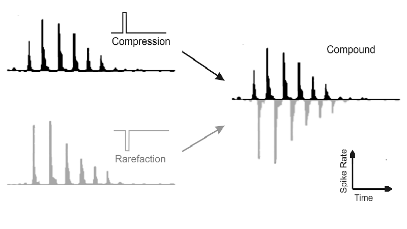
Figure 2.12
Responses of a low-frequency
AN fiber to compression or rarefaction clicks, shown as PSTHs.
Basilar membrane ringing causes multiple peaks in the neural discharge in
response to a single click. The combined response to compression and
rarefaction clicks resembles the impulse response of a gamma-tone filter. Based
on data collected by Goblick and Pfeiffer (1969)
So if individual auditory nerve
fibers respond approximately like gamma-tone filters, as figure
2.12 suggests, then groups of nerve fibers ought to
represent sounds in a manner very much like the cochleagram
gamma-tone filter bank we had encountered in figure 2.6.
That this is indeed the case is beautifully illustrated by a set of auditory
nerve fiber responses recorded by Bertrand Delgutte (1997),
and reproduced here in figure 2.13.
The nerve fiber responses were recorded in the auditory nerve of an
anesthetized cat, and are shown in figure 2.13A
as histograms, arranged by each neuron’s characteristic frequency, as shown to
the left. Below the histograms, in figure 2.13B,
you can see the spectrogram of the sound stimulus, the recording of a spoken
sentence.
When you compare the spectrogram
to the neural responses, you will notice a clear and straightforward
relationship between the sound energy and neural firing rate distributions.
During the quiet periods in the acoustic stimulus, the nerve fibers fire at
some low, spontaneous background rate, but as soon as the stimulus contains
appreciable amounts of acoustic energy near the nerve fiber’s characteristic
frequency, firing rates increase substantially, and the greater the sound
intensity, the greater the firing rate increase. The firing rate distribution
across this population of auditory nerve fibers has produced a neurogram representation of the incoming sounds in the
auditory nerve. This neurogram in many ways resembles
the short-time spectrogram of the presented speech, and shows formants in the
speech sound very clearly.
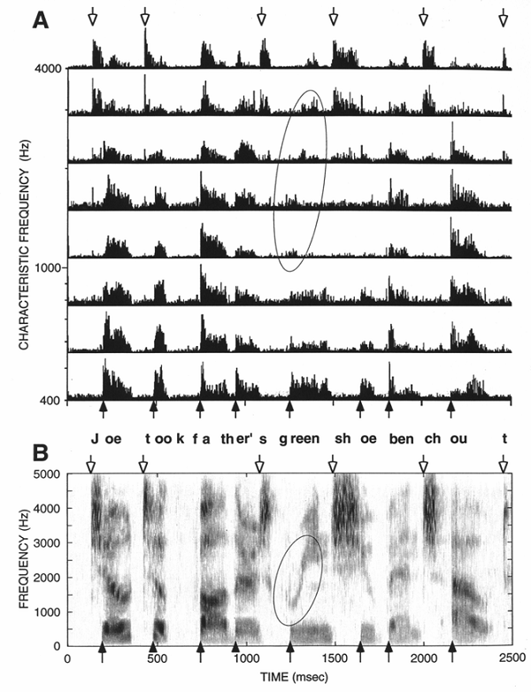
Figure 2.13
(A) Neurogram of the spoken sentence, “Joe took father’s green
shoe bench out.” Poststimulus time histograms of the firing rates of auditory nerve fibers,
arranged by each nerve fiber’s characteristic frequency. (B) Spectrogram
of the spoken sentence shown for comparison. The ellipses are to emphasize that
even fine details, like the rapid formant transition in “green,” are represented
in the dynamic changes of the auditory nerve firing rates.
From Delgutte
(1997), Handbook of Phonetic Sciences (Laver, ed), pp 507-538.
The neurogram
representation in figure 2.13 relies on two basic properties
of auditory nerve fibers: first, that they are frequency tuned, and second,
that their firing rate increases monotonically with increases in sound level.
All of these properties arise simply from the excitatory, synaptic coupling
between inner hair cells and auditory nerve fibers. But the synapses linking
inner hair cells to auditory nerve fibers appear not to be all the same.
You may recall that each inner
hair cell is connected to approximately twenty type I fibers. Why so many? Part
of the answer is probably that more fibers allow a more precise representation
of the sound, as encoded in the inner hair cell’s membrane voltage. Spike
trains are in a sense binary: Nerve fibers, those of the auditory nerve
included, are subject to refractory periods, meaning that once they have fired
an action potential, they are incapable of firing another for at least 1 ms.
Consequently, no neuron can fire at a rate greater than 1 kHz or so, and indeed
few neurons appear capable of maintaining firing rates greater than about 600
Hz for any length of time. Consequently, during any short time interval of a
millisecond or 2, a nerve fiber either fires an action potential or it does
not, which might signal that the sound pressure at the neuron’s preferred
frequency is large, or that it is not. Of course, if you have several fibers at
your disposal, you can start to send more detailed information. You might, for
example, signal that the sound pressure is sort of intermediate, neither very
small nor very large, by firing a proportion of the available nerve fibers that corresponds to the strength of the signal. Or
you could reserve some nerve fibers exclusively for signaling intense sounds,
while others might fire like crazy at the slightest whisper of a sound.
This second option seems to be the
one adopted by your auditory nerve. The connections on the modiolar
side of the hair cell seem to be less excitable than those facing toward the
outside of the cochlear spiral (Liberman, 1982). Nerve
fibers connected on the outward-facing side therefore respond even to the
quietest sounds, but their firing rates easily saturate, so that at even
moderate sound levels of around 30 to 50 dB SPL they fire as fast as they can,
and their firing rates cannot increase further with further increases in sound
pressure. These highly excitable nerve fibers also have elevated spontaneous
firing rates. They fire as many as 20 to 50 spikes or more a second in complete
quiet, and they are consequently often referred to as high spontaneous rate
fibers. The fibers connected to the inward-facing, modiolar
side of the inner hair cells, in contrast, are known either as medium
spontaneous rate fibers if they fire less than 18 spikes/s in silence, or as
low spontaneous rate fibers, if their spontaneous firing rates are no more than
about 1 spike/s. Medium and low spontaneous rate fibers tend not to increase
their firing rate above this background rate until sound levels reach at least some
20 to 30 dB SPL, and their responses tend not to saturate until sound levels
reach 80 dB SPL or more. The acoustically more sensitive, high spontaneous rate
fibers, appear to be more numerous, outnumbering the
low spontaneous rate fibers by about 4 to 1.
Now, the information that these
nerve fibers encode about incoming sounds is, as we had already mentioned,
relayed to them from sounds encoded as hair cell membrane potentials via
excitatory synapses. You may remember from figure 2.9
that hair cell membrane potentials will encode low frequencies faithfully as
analog, AC voltage signals, but for frequencies higher than a few kilohertz, they
switch into a DC mode, in which membrane voltage depolarizes with increasing
sound level but does not follow individual cycles of the stimulus waveform.
This behavior of inner hair cells is also reflected in the firing of the
auditory nerve fibers to which they connect. At low frequencies, as the inner
hair cell membrane potential oscillates up and down in phase with the incoming
sound, the probability of transmitter release at the synapses, and hence the
probability of action potential firing of the nerve fiber, also oscillate in
step. For low stimulus frequencies, auditory nerve fibers therefore exhibit a
phenomenon known as “phase locking,” which is illustrated in figure
2.14. (There is also a classic video clip from the
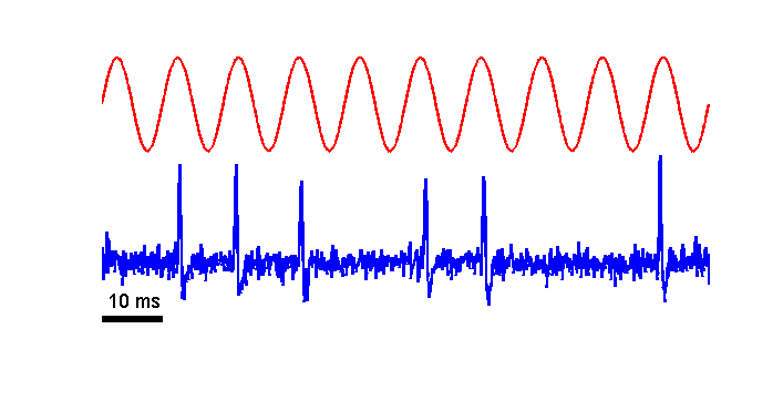
Figure 2.14
Simulation of an
auditory nerve fiber recording (black line) in response to a 100-Hz tone (gray
line).
Figure 2.14 shows a simulation of an
extracellular recording of an auditory nerve fiber response (black) to a 100-Hz
sine wave (gray). You may observe that the spikes tend to occur near the crest
of the wave, when the stereocilia of the hair cells
are most deflected, the depolarization of the hair cells is greatest, and the
rate of neurotransmitter release is maximal. However, it is important to note
that this phase locking, meaning the synchronization of the spikes with
the crest of the sound stimulus is not a process with clockwork precision.
First of all, the spikes do not occur on every crest. This is important if we
want to have phase locking but also a spike rate representation of sound
intensity. During quiet sounds, a nerve fiber may skip most of the sine wave
cycles, but as it gets louder, the fiber skips fewer and fewer cycles, thereby
increasing its average firing rate to signal the louder sound. In fact, for
very quiet, near-threshold sounds, nerve fibers may not increase their firing
rates at all above their spontaneous rate, but merely signal the presence of
the sound because their discharges no longer occur at random, roughly Poisson
distributed intervals, but achieve a certain regularity due to phase locking.
Also note that the spikes are most likely to occur near the crest of the wave, but
they are not guaranteed to occur precisely at the top. Action potentials during
the trough of the wave are not verboten, they are just less likely.
The phase locking of a nerve fiber
response is said to be stochastic, to underline the residual randomness that
arises because nerve fibers may skip cycles and because their firing is not precisely
time-locked to the crest of the wave. The timing of a single action potential
of a single fiber is therefore not particularly informative, but if you can
collect enough spikes from a number of nerve fibers, then much can be learned
about the temporal fine structure of the sound from the temporal distribution
of the spikes. Some authors use the term “volley principle” to convey the idea
that, if one nerve fiber skips a particular cycle of sound stimulus, another neighboring
nerve fiber may mark it with a nerve impulse. This volley principle seems to
make it possible for the auditory nerve to encode temporal fine structure at
frequencies up to a few kilohertz, even though no single nerve fiber can fire
that fast, and most fibers will have to skip a fair
proportion of all wave crests.
There is no evidence at present
that auditory nerve fibers use any particularly sophisticated mechanism to take
turns in firing phase-locked volleys, but they probably don’t need to. Bearing
in mind that each inner hair cell connects to about two dozen nerve fibers, and
that the inner hair cells immediately on either side of it must experience
virtually identical vibrations, as they sit on more or less the same patch of
the basilar membrane, the number of nerve fibers available to provide
potentially phase-locked information in any one frequency channel is
potentially quite large, perhaps in the hundreds. And there is a lot of
evidence that the brain uses the temporal fine structure information conveyed
in the spike timing distribution of these fibers in several important auditory
tasks, including musical pitch judgments (as we shall see in chapter 3) or the
localization of sound sources (as we shall see in chapter 5).
Of course, since phase locking in
the auditory nerve fibers depends on inner hair cells operating in AC mode, we
cannot expect them to phase lock to frequencies or temporal patterns faster
than a few kilohertz. That this is, indeed, so has already been demonstrated in
auditory nerve fiber recordings conducted many decades ago. Figure
2.15 is based on recordings from an auditory nerve fiber
of an anesthetized squirrel monkey, carried out by Rose and colleagues in 1967.
Responses to 1,000-, 2,000-, 2,500-, 3,000- and 4,000 Hz tones are shown. The
responses are displayed as period histograms. Period histograms show the
number, or the proportion, of action potentials that occur during a particular
phase of the stimulus cycle.
In response to the 1,000
Hz sound, the responses were quite obviously phase locked, as a clear majority
of spikes happened halfway through the cycle, i.e. ca 180º (π radians) out
of phase with the stimulus. (Note that the phase of the stimulus here is
determined at the eardrum, and given the phase delays that occur between eardrum
and auditory nerve fiber, phase-locked responses need not occur at 0º.) This
peak in the period histogram is most obvious in response to the 1,000-Hz tone
shown, still quite clear at 2,000 and 2,500 Hz, but definitely on the way out
at 3,000 Hz and completely gone at 4,000 Hz.
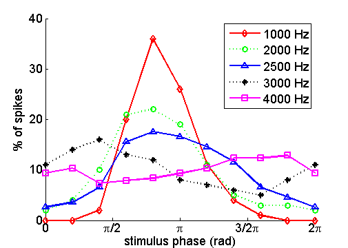
Figure 2.15
Period histograms of
responses to pure tones recorded from an auditory nerve fiber in a squirrel
monkey. The traces show the proportion of action potentials fired at a
particular phase of a pure tone stimulus. The stimulus frequency is indicated
in the legend. Based on data
collected by Rose et al. (1967).
One thing to point out in the
context of figure 2.15 is that it is clearly the
frequency content of the sound that determines whether an auditory nerve fiber
will phase lock, not the fiber’s characteristic frequency. All traces in figure
2.15 show data recorded from one and the same nerve fiber,
which happened to have a characteristic frequency of approximately 4,000 Hz.
You may be surprised that this 4-kHz fiber, although it is unable to phase lock
to tones at its own characteristic frequency, not only clearly responds to 1-kHz
sounds, a full two octaves away from its own CF, but also phase locks
beautifully at these lower frequencies. But bear in mind that the nerve fiber’s
responses simply reflect both the mechanics of the basilar membrane and the
behavior of inner hair cells.
We saw earlier (figure
2.10) that the mechanical tuning of the basilar membrane
becomes very broad when stimulated with fairly loud sounds. Consequently,
auditory nerve fibers will often happily respond to frequencies quite far
removed from their CF, particularly on the lower side, provided these sounds
are loud enough. And the AC hair cell responses that are the basis of phase
locking appear to occur in similar ways in inner hair cells all along the
cochlea. Thus, when we say, on the basis of data like those shown in figure
2.15 and further recordings by many others, that mammals have
a phase locking limit somewhere around 3 to 4 kHz, this does not mean that we
cannot occasionally observe stimulus-locked firing patterns in neurons that are
tuned to frequencies well above 4 kHz. If we stimulate a very sensitive 5-kHz
fiber with a very loud 2-kHz tone, we might well observe a response that phase
locks to the 2-kHz input. Or we might get high-frequency fibers to phase lock
to temporal “envelope patterns,” which ride on the high frequencies. Imagine
you were to record from a nerve fiber tuned to 10 kHz and present not a single
tone, but two tones at once, one of 10 kHz, the other of 10.5 kHz. Since the
two simultaneous tones differ in frequency by 500 Hz, they will go in and out
of phase with each other 500 times a second, causing rapid cycles of
alternating constructive and destructive interference known as “beats.” It is a
bit as if the 10-kHz tone was switched on and off repeatedly, 500 times a
second. Auditory nerve fibers will respond to such a sound, not by phase
locking to the 10-kHz oscillation, as that is too high for them, but by phase
locking to the 500 Hz beat, the rapid amplitude modulation of this sound. This
sort of envelope phase locking to amplitude modulations of a high-frequency
signal is thought to be, among other things, an important cue for pitch
perception, as we will see in chapter 3.
2.6 Stations of the Central Auditory Pathway
We end this chapter
with a whirlwind tour of the main stations of the ascending auditory pathway.
The anatomy of the auditory pathway is extraordinarily complicated, and here we
will merely offer a very rough overview of the main processing stations and
connections, to orient you and help you embed the discussions in the later
chapters in their anatomical context. With that in mind, let us briefly run
through the route that acoustic information takes as it travels from the
cochlea all the way to the very highest processing centers of your brain.
Upon leaving the cochlea, the
auditory nerve fibers join the VIII cranial (vestibulocochlear)
nerve and enter the cochlear nucleus (CN) in the brainstem. There, they
immediately bifurcate. One ascending branch enters the anteroventral
cochlear nucleus (AVCN); the other descending branch runs through the posteroventral (PVCN) to the dorsal cochlear nucleus (DCN).
Each nerve fiber branch forms numerous synapses with the many distinct types of
neurons that populate each of the three subdivisions of the CN. CN neurons come
in different characteristic types, which differ in their anatomical location, morphology,
cellular physiology, synaptic inputs, and temporal and spectral response
properties, as illustrated in figure 2.16.
For example, the AVCN contains
so-called spherical and globular bushy cells, which receive a very small number
of unusually large, strong, excitatory synapses (the so-called endbulbs of Held) from the auditory nerve fibers. Bushy
cells are said to exhibit primary-like responses, which is just a short way of
saying that the synaptic coupling between bushy cells and the auditory nerve
fibers is so tight that the firing patterns in bushy cells in response to sound
are very similar to those in the auditory nerve fibers that drive them.
Consequently, they accurately preserve any information carried in the temporal
firing patterns of the auditory nerve fibers. Another cell type that can be
found in the AVCN and also in the PVCN is the stellate
(i.e., star-shaped) cell, which receives convergent inputs from several
auditory nerve fibers as well as from other types of neurons. Physiologically, stellate cells of the AVCN are mostly chopper
cells, which means they tend to respond to pure-tone stimuli with
regular, rhythmic bursts, in which the burst frequency appears to be unrelated
to that of the tone stimuli. Thus, these neurons do not preserve the timing of
their input spikes, but they tend to have narrower frequency tuning, and
possibly also a larger dynamic range, than their auditory nerve inputs. This
may make them better suited for coding details of the spectral shape of the
incoming stimuli.
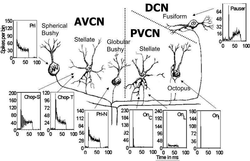
Figure 2.16
Cell types of the
cochlear nucleus. Pri, primarylike;
Pri-N, primarylike with
notch; Chop-S, chopper sustained; Chop-T, chopper transient; OnC, onset chopper; OnL, onset locker; OnI, onset inhibited.
Adapted from
original artwork by Prof. Alan Palmer, with kind permission.
In the PVCN, one frequently finds onset
cells that respond to pure-tone bursts with just a single action potential at
the start of the sound. Morphologically, these onset cells are either stellate (with somewhat different intrinsic properties than
the choppers), or octopus shaped. They receive convergent input from many
auditory nerve fibers and are therefore very broadly frequency tuned. While
they mark the onset of pure tones with great accuracy (their response latency
jitter is in the range of tens of microseconds), it would nevertheless be
misleading to think of the purpose of these cells as only marking the beginning
of a sound. In fact, if these cells are stimulated with complex tones, for
example, a 300-Hz and a 400-Hz tone played together so that they would beat
against each other 100 times a second, then the onset cells would mark not just
the beginning of this complex tone, but every beat, with an action potential.
These cells may therefore provide much more detail about the time structure of
a complex tone than the term “onset cell” would suggest. In contrast, cells in
the DCN, which have more complex, “pauser” type
temporal response patterns and can have a “fusiform” (or
“pyramidal”) morphology, exhibit responses that are often characterized by being
inhibited by some frequencies, as well as excited by others. Thus, while VCN
cells may be specialized for processing the temporal structure of sounds, DCN
cells may thus play a particular role in detecting spectral contrasts. To make
all of this even more perplexing, the DCN receives, in addition to its auditory
inputs, some somatosensory input from the skin. Note
that cognoscenti of the cochlear nucleus distinguish further subtypes among the
major classes we have just discussed, such as chopper-transients or onset-lockers
or primary-like with notch, but a detailed discussion of these distinctions
would lead us too far.
The various principal cell types
in the CN also send their outputs to different parts of the ascending auditory
pathway. The major stations of that pathway are illustrated schematically in figure
2.17. All (or almost all) of the outputs from the CN will
eventually reach the first major acoustic processing station of the midbrain,
the inferior colliculus (IC), but while most stellate and most DCN cells send axons directly to the IC,
the outputs from AVCN bushy cells take an indirect route, as they are first
relayed through the superior olivary complex (SOC) of
the brainstem. At the olivary nuclei, there is convergence
of a great deal of information from the left and right ears, and these nuclei
make key contributions to our spatial (stereophonic) perception of sound. We
will therefore revisit the SOC in some detail when we discuss spatial hearing
in chapter 5.
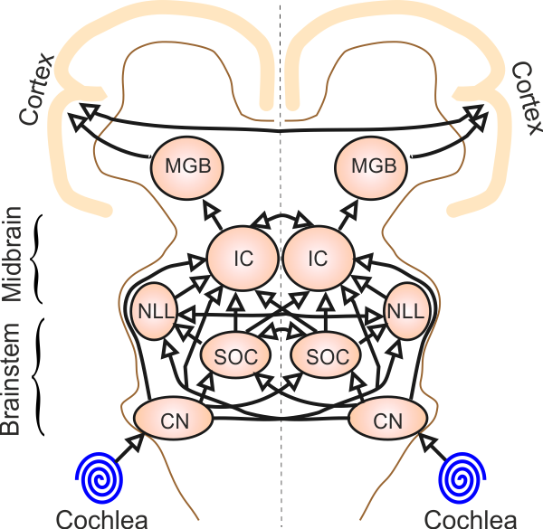
Figure 2.17
Simplified
schematic diagram of the ascending auditory pathway. CN, cochlear
nuclei; SOC, superior olivary complex; NLL, nuclei of
the lateral lemniscus; IC, inferior colliculus; MGB, medial geniculate
body.
Axons from the cochlear and olivary nuclei then travel along a fiber bundle known as
the lateral lemniscus to the IC. On the way, they may
or may not send side branches to the ventral, intermediate or dorsal nuclei of
the lateral lemniscus (NLL). Note that the paths from
CN to the IC are predominantly crossed, and indeed, neurons in the midbrain and
cortex tend to be most strongly excited by sounds presented to the opposite, contralateral ear.
The IC itself has a complex
organization, with a commissural connection between the left and right IC that allows
for yet further binaural interactions within the ascending pathway. There are
also numerous interneurons within the IC, which
presumably perform all manner of as yet poorly understood operations. The IC is
subdivided into several subnuclei. The largest, where
most of the inputs from the brainstem arrive, is known as the central nucleus
of the IC (ICc), and it is
surrounded by the dorsal nucleus (ICd) at the top,
the external nucleus (ICx), and the nucleus of the
brachium of the IC (BIC) at the front. The BIC sends axons to an eye movement
control center known as the superior colliculus (SC),
to enable reflexive eye movements toward unexpected sounds. However, most of
the axons leaving the nuclei of the IC travel through the fiber bundle of the
brachium toward the major auditory relay nucleus of the thalamus, the medial geniculate body (MGB). The MGB, too, has several distinct
subdivisions, most notably ventral (MGv),
dorsal (MGd),
and medial (MGm).
Note that the CN, the OC, the NLL, as well as the ICc and the MGv all
maintain a clear tonotopic organization, that is,
neurons within these neurons are more or less sharply frequency tuned and
arranged anatomically according to their best frequency. Thus, in the ICc, for example, neurons tuned to
low frequencies are found near the dorsal surface and neurons of increasingly
higher frequency are found at increasingly deeper, more ventral locations. In
contrast, the ICx, BIC, and MGd
lack a clear tonotopic order. Tonotopically
organized auditory midbrain structures are sometimes referred to as “lemniscal,” and those that lack tonotopic
order as “paralemniscal.”
Some thalamic output fibers from
the MGB then connect to limbic structures of the brain, such as the amygdala, which is thought to coordinate certain types of
emotional or affective responses and conditioned reflexes to sound, but the
large majority of fibers from the thalamus head for the auditory cortex in the
temporal lobes. The auditory cortical fields on either side are also
interconnected via commissural connections through the corpus callosum, providing yet another opportunity for an exchange
of information between left and right, and, indeed, at the level of the
auditory cortex, the discharge patterns of essentially all acoustically
responsive neurons can be influenced by stimuli delivered to either ear.
The auditory cortex, too, is
subdivided into a number of separate fields, some of which show relatively
clear tonotopic organization,
and others less so. Apart from their tonotopy, different cortical fields are
distinguished by their anatomical connection patterns (how strong a projection they
receive from which thalamic nucleus, and which brain regions they predominantly
project to), physiological criteria (whether neurons are tightly frequency
tuned or not, respond at short latencies or not, etc.) or their content of
certain cell-biological markers, such as the protein parvalbumin.
Up to and including the level of the thalamus, the organization of the
ascending auditory pathway appears to be fairly stereotyped among most if not all
species of mammals. There are some differences; for example, rats have a
particularly large intermediate NLL, cats a particularly well-developed lateral
superior olivary nucleus, and so on, but cats, rats,
bats, and monkeys nevertheless all have a fundamentally similar organization of
subcortical auditory structures, and anatomically
equivalent structures can be identified without too much trouble in each
species. Consequently, the anatomical names we have encountered so far apply
equally to all mammals. Unfortunately, the organization of auditory cortical
fields may differ from one species of mammal to the next, particularly in
second- or third-order areas, and very different names are used to designate
cortical fields in different species. We illustrate the auditory cortex of
ferrets, cats, and monkeys in figure 2.18.
Note that the parcellations shown in figure 2.18
are based in large part on anatomical tract tracer injection and extracellular
recording studies, which cannot readily be performed in humans, and our
understanding of the organization of human auditory cortex therefore remains
fairly sketchy, but we will say a bit more about this in chapter 4 when we
discuss the processing of speech sounds.
It may be that some of the fields
that go by different names in different species actually have rather similar functions,
or common evolutionary histories. For example, both carnivores and primates
have two primary cortical areas, which lie
side-by-side and receive the heaviest thalamic input; but while these fields
are called A1 and AAF (for anterior auditory field) in carnivores, they are
designated as A1 and R in monkeys. To what extent AAF and R are really equivalent
is uncertain. Similarly, the cat’s posterior auditory field (P, or PAF) may or
may not be equivalent to the ferret’s PSF and PPF, or the monkey’s areas CL and
CM,. It is easily possible, perhaps even likely, that
there may be quite fundamental differences in the organization of auditory cortex
of different species. The cortex is after all the youngest and most malleable
part of the brain in evolutionary terms. Thus, the auditory cortex of echolocating bats features a number of areas that appear to
be specialized for the processing of echo delays and Doppler shifts for which
there is no obvious equivalent in the brain of a monkey.
Figure 2.18
Drawings showing identified auditory cortical areas in the ferret (A), the cat (B) and the rhesus macaque (C). Primary areas are shown in dark gray, higher-order (belt and parabelt) areas in light gray.
What seems to be true for all mammals,
though, is that one can distinguish primary and second-order (belt) areas of
auditory cortex, and these interact widely with the rest of the brain,
including the highest-order cognitive structures, such as pre-frontal lobe areas
thought to be involved in short-term memory and action planning, or the infratemporal structures thought to mediate object
recognition. To the best of our knowledge, without these very high level
cortical areas, we would be unable to recognize the sound of a squealing car
tire, or to remember the beginning of a spoken sentence by the time the
sentence is concluded, so they, too, are clearly integral parts of the auditory
brain.
Our whirlwind tour of the auditory
pathway has, thus, finally arrived at the very highest levels of the mammalian
brain, but we do not want to leave you with the impression that in this pathway
information only flows upwards, from the cochlear toward the cortex. There are
also countless neurons relaying information back down, from frontal cortex to
auditory cortex, from auditory cortex to the MGB and the IC, and from the IC to
the CN as well as to the so-called periolivary
nuclei, which in turn send axons back out through the VIII cranial nerve to
synapse with the outer hair cells of the cochlea. This anatomical arrangement
indicates that auditory processing does not occur in a purely feedforward fashion. It can incorporate feedback loops on
many levels, which make it possible to retune the system on the fly, right down
to the level of the mechanics of the cochlea, to suit the particular demands the
auditory system faces in different environments or circumstances.