1
Why Things Sound the Way They Do
- 1.1 Simple Harmonic Motion—Or, Why Bells Go “Bing” When You Strike Them
- 1.2 Modes of Vibration and Damping—Or Why a “Bing” Is Not a Pure Tone
- 1.3 Fourier Analysis and Spectra
- 1.4 Windowing and Spectrograms
- 1.5 Impulse Responses and Linear Filters
- 1.6 Voices
- 1.7 Sound Propagation
- 1.8 Sound Intensity
We are very fortunate
to have ears. Our auditory system provides us with an incredibly rich and nuanced
source of information about the world around us. Listening is not just a very
useful, but also often a very enjoyable activity. If your ears, and your
auditory brain, work as they should, you will be able to distinguish thousands
of sounds effortlessly—running water, slamming doors, howling wind, falling
rain, bouncing balls, rustling paper, breaking glass, or footsteps (in fact,
countless different types of footsteps: the crunching of leather soles on
gravel, the tic-toc-tic of stiletto heels on a marble floor, the cheerful
splashing of a toddler stomping through a puddle, or the rhythmic drumming of
galloping horses or marching armies). The modern world brings modern sounds.
You probably have a pretty good idea of what the engine of your car sounds
like. You may even have a rather different idea of what the engine of your car ought to sound like, and be concerned
about that difference. Sound and hearing are also enormously important to us
because of the pivotal role they play in human communication. You have probably
never thought about it this way, but every time you talk to someone, you are
effectively engaging in something that can only be described as a telepathic
activity, as you are effectively “beaming your thoughts into the other person’s
head,” using as your medium a form of “invisible vibrations.” Hearing, in other
words, is the telepathic sense that we take for granted (until we lose it) and
the sounds in our environment are highly informative, very rich, and not rarely
enjoyable (and we haven’t even mentioned music yet!)
If you have read other
introductory texts on hearing, they will probably have told you, most likely
right at the outset, that “sound is a pressure wave, which propagates through
the air.” That is, of course, entirely correct, but it is also somewhat missing
the point. Imagine you hear, for example, the din of a drawer full of cutlery
crashing down onto the kitchen floor. In that situation, lots of minuscule
ripples of air pressure will be radiating out from a number of mechanically
excited metal objects, and will spread outwards in concentric spheres at the
speed of sound, a breathless 340 m/s (about 1,224 km/h or 760 mph), only to
bounce back from the kitchen walls and ceiling, filling, within only a few
milliseconds, all the air in the kitchen with a complex pattern of tiny, ever
changing ripples of air pressure. Fascinating as it may be to try to visualize
all these wave patterns, these sound waves certainly do not describe what we
“hear” in the subjective sense.
The mental image your sense of
hearing creates will not be one of delicate pressure ripples dancing through
the air, but rather the somewhat more alarming one of several pounds of sharp
knives and forks, which have apparently just made violent and unexpected contact
with the kitchen floor tiles. Long before your mind has had a chance to ponder
any of this, your auditory system will already have analyzed the sound pressure
wave pattern to extract the following useful pieces of information: that the
fallen objects are indeed made of metal, not wood or plastic; that there is
quite a large number of them, certainly more than one or two; that the fallen
metal objects do not weigh more than a hundred grams or so each (i.e., the
rampaging klutz in our kitchen has indeed spilled the cutlery drawer, not
knocked over the cast iron casserole dish); as well as that their impact
occurred in our kitchen, not more than 10 meters away, slightly to the left,
and not in the kitchen of our next door neighbors or in a flat overhead.
That our auditory brains can
extract so much information effortlessly from just a few “pressure waves” is
really quite remarkable. In fact, it is more than remarkable, it is
astonishing. To appreciate the wonder of this, let us do a little thought
experiment and imagine that the klutz in our kitchen is in fact a “compulsive
serial klutz,” and he spills the cutlery drawer not once, but a hundred times,
or a thousand. Each time our auditory system would immediately recognize the
resulting cacophony of sound: “Here goes the cutlery drawer again.” But if you
were to record the sounds each time with a microphone and then look at them on
an oscilloscope or computer screen, you would notice that the sound waves would
actually look quite different on each and every occasion.
There are infinitely many
different sound waves that are all recognizable as the sound of cutlery
bouncing on the kitchen floor, and we can recognize them even though we hear
each particular cutlery-on-the-floor sound only once in our lives. Furthermore,
our prior experience of hearing cutlery crashing to the floor is likely to be
quite limited (cutlery obsessed serial klutzes are, thankfully, a very rare
breed). But even so, most of us have no difficulty imagining what cutlery
crashing to floor would sound like. We can even imagine how different the sound
would be depending on whether the floor was made of wood, or covered in
linoleum, or carpet, or ceramic tiles.
This little thought experiment
illustrates an important point that is often overlooked in introductory texts
on hearing. Sound and hearing are so useful because things make sounds, and different things make different sounds.
Sound waves carry valuable clues about the physical properties of the objects
or events that created them, and when we listen we do not seek to sense
vibrating air for the sake of it, but rather we hope to learn something about
the sound sources, that is, the
objects and events surrounding us. For a proper understanding of hearing, we
should therefore start off by learning at least a little bit about how sound
waves are created in the first place, and how the physical properties of sound
sources shape the sounds they make.
1.1 Simple Harmonic Motion—Or, Why Bells Go “Bing” When You Strike Them
Real-world sounds,
like those we just described, are immensely rich and complex. But in sharp
contrast to these “natural” sounds, the sounds most commonly used in the
laboratory to study hearing are by and large staggeringly dull. The most common
laboratory sound by far is the sine wave pure tone, a sound
which most nonscientists would describe, entirely accurately, as a “beep”—but
not just any beep, and most certainly not an interesting one. To be a “pure”
tone, the beep must be shorn of any “contaminating” feature, be completely
steady in its amplitude, contain no “amplitude or frequency modulations”
(properties known as vibrato to the
music lover) nor any harmonics (overtones) or other embellishing features. A
pure tone is, indeed, so bare as to be almost “unnatural”: pure tones are
hardly ever found in everyday soundscapes, be they manmade or natural.
You may find this puzzling. If
pure tones are really quite boring and very rare in nature (and they are
undeniably both), and if hearing is about perceiving the real world, then why
are pure tones so widely used in auditory research? Why would anyone think it a
good idea to test the auditory system mostly with sounds that are neither
common nor interesting? There are, as it turns out, a number of reasons for
this, some good ones (or at least they seemed good at the time) and some
decidedly less good ones. And clarifying the relationship between sinusoidal
pure tones and “real” sounds is in fact a useful, perhaps an essential, first
step toward achieving a proper understanding of the science of hearing. To take
this step we will need, at times, a mere smidgen of mathematics. Not that we
will expect you, dear reader, to do any math yourself, but we will encourage
you to bluff your way along, and in doing so we hope you will gain an intuitive
understanding of some key concepts and techniques. Bluffing one’s way through a
little math is, in fact, a very useful skill to cultivate for any sincere
student of hearing. Just pretend that you kind of know this and that you only
need a little “reminding” of the key points. With that in mind, let us
confidently remind ourselves of a useful piece of applied mathematics that goes
by the pleasingly simple and harmonious name of simple harmonic motion. To develop an intuition for this, let us
begin with a simple, stylized object, a mass spring system, which consists of a
lump of some material (any material you like, as long as it’s not weightless
and is reasonably solid) suspended from an elastic spring, as shown in figure 1.1. (See the book’s website for an
animated version of this figure <flag>).
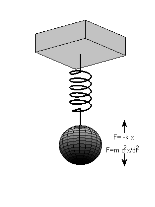
Figure 1.1
A mass spring system.
Let us also imagine that this
little suspended mass has recently been pushed, so that it now travels in a
downward direction. Let us call this the x
direction. Now is an excellent time to start pretending that we were once quite
good at school math and physics, and, suitably reminded, we now recall that
masses on the move are inert, that is, they have a tendency to keep on moving
in the same direction at the same speed until something forces them to slow
down or speed up or change direction. The force required to do that is given by
Newton’s second law of motion, which states that force equals mass times
acceleration, or F = m ∙ a.
Acceleration, we further recall,
is the rate of change of velocity (a=dv/dt)
and velocity is the rate of change of position (v=dx/dt). So we can apply Newton’s second law to our little mass as
follows: It will continue to travel with constant velocity dx/dt in the x direction
until it experiences a force that changes its velocity; then the rate of change
in velocity is given by F = m ∙ d2x/dt2.
(By the way, if this is getting a bit heavy going, you may skip ahead to the
paragraph beginning “In other words… .” We won’t tell anyone you skipped ahead,
but note that bluffing your way in math takes a little practice, so persist if
you can.) Now, as the mass travels in the x
direction, it will soon start to stretch the spring, and the spring will start
to pull against this stretch with a force given by Hooke’s law, which states
the pull of the spring is proportional to how far it is stretched, and it acts
in the opposite direction of the stretch (i.e., F = - k ∙x, where k
is the spring constant, a proportionality factor that is large for strong,
stiff springs and small for soft, bendy ones; the minus sign reminds us that
the force is in a direction that opposes further stretching).
So now we see that, as the mass
moves inertly in the x direction,
there soon arises a little tug of war, where the spring will start to pull
against the mass’ inertia to slow it down. The elastic force of the spring and
the inertial force of the mass are then, in accordance with Newton’s third law
of motion, equal in strength and opposite in direction, that is, -k ∙ x = m ∙ d2x/dt2.
We can rearrange this equation using elementary algebra to d2x/dt2 = -k/m ∙ x to obtain something that many students of psychology
or biology would rather avoid, as it goes by the intimidating name of second-order differential equation. But
we shall not be easily intimidated. Just note that this equation only
expresses, in mathematical hieroglyphics, something every child playing with a
slingshot quickly appreciates intuitively, namely, that the harder one pulls
the mass in the slingshot against the elastic, the harder the elastic will try
to accelerate the mass in the opposite direction. If that rings true, then
deciphering the hieroglyphs is not difficult. The acceleration d2x/dt2 is large
if the slingshot has been stretched a long way (-x is large), if the slingshot elastic is stiff (k is large), and if the mass that needs
accelerating is small (again, no surprise: You may remember from childhood that
large masses, like your neighbor’s garden gnomes, are harder to catapult at
speed than smaller masses, like little pebbles).
But what does all of this have to
do with sound? This will become clear when we quickly “remind” ourselves how
one solves the differential equation d2x/dt2
= -k/m ∙ x. Basically, here’s how
mathematicians do this: they look up the solution in a book, or get a computer
program for symbolic calculation to look it up for them, or, if they are very
experienced, they make an intelligent guess and then check if it’s true.
Clearly, the solution must be a function that is proportional to minus its own
second derivative (i.e., “the rate of change of the rate of change” of the
solution must be proportional to minus its current value). It just so happens
that sine and cosine functions, pretty much uniquely, possess this property.
Look at the graph of the cosine function that we have drawn for you in figure 1.2, and note that, at zero, the cosine
has a value of 1, but is flat because it has reached its peak, and has
therefore a slope of 0. Note also that the -sine function, which is also
plotted in gray, has a value of 0 at zero, so here the slope of the cosine
happens to be equal to the value of -sine. This is no coincidence. The same is
also true for cos(π/2), which happens to have a value of 0 but is falling
steeply with a slope of -1, and -sin(π/2) is also -1. It is, in fact, true
everywhere. The slope of the cosine is minus the sine, and the slope of minus
sine is minus the cosine. Sine waves, uniquely, describe the behavior of mass
spring systems, because they are everywhere proportional to minus their own
second derivative [d2
cos(t)/dt2 = -cos(t)] and they therefore satisfy the
differential equation that describes the forces in a spring-mass system.
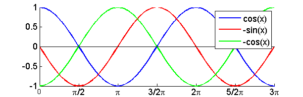
Figure 1.2
The cosine and its
derivatives.
In other words, and this is the
important bit, the natural behavior for
any mass spring system is to vibrate in a sinusoidal fashion. And given
that many objects, including (to get back to our earlier example) items of
cutlery, have both mass and a certain amount of springiness, it is perfectly
natural for them, or parts of them, to enter into “simple harmonic motion,”
that is, to vibrate sinusoidally. Guitar or piano strings, bicycle bells,
tuning forks, or xylophone bars are further familiar examples of everyday mass
spring systems with obvious relevance to sound and hearing. You may object that
sinusoidal vibration can’t really be the “natural way to behave” for all mass
spring systems, because, most of the time, things like your forks and knives do
not vibrate, but sit motionless and quiet in their drawer, to which we would
reply that a sinusoidal vibration of zero amplitude is a perfectly fine
solution to our differential equation, and no motion at all still qualifies as
a valid and natural form of simple harmonic motion.
So the natural behavior (the
“solution”) of a mass spring system is a sinusoidal vibration, and written out
in full, the solution is given by the formula x(t) = xo · cos(t · √(k/m)+φo), where xo is the
“initial amplitude” (i.e., how far the little mass had been pushed downward at
the beginning of this little thought experiment), and φo is its “initial phase” (i.e., where it was in
the cycle at time zero). If you remember how to differentiate functions like
this, you can quickly confirm that this solution indeed satisfies our original
differential equation. Alternatively, you can take our word for it. But we
would not be showing you this equation, or have asked you to work so hard to
get to it, if there weren’t still quite a few very worthwhile insights to gain
from it. Consider the cos(t · √(k/m)) part. You may remember that the cosine
function goes through one full cycle over an angle of 360o, or 2π radians. So the mass spring
system has swung through one full cycle when t · √(k/m)
equals 2π. It follows that the period (i.e., the time taken for one
cycle of vibration) is T = 2π/√(k/m). And you may recall that the frequency (i.e., the number of cycles per
unit time) is equal to 1 over the period, so f = √(k/m)/2π.
Translated into plain English,
this tells us that our spring mass system has a preferred or natural frequency
at which it wants to oscillate or vibrate. This frequency is known as the
system’s resonance frequency, and it is inversely proportional
to its mass and proportional to the square root of its stiffness. If this
frequency lies within the human audible frequency range (about 50–20,000
cycles/s, or Hz), then we may hear these vibrations as sound. Although you may,
so far, have been unaware of the underlying physics, you have probably
exploited these facts intuitively on many occasions. So when, to return to our
earlier example, the sounds coming from our kitchen tell us that a box full of
cutlery is currently bouncing on the kitchen floor, we know that it is the
cutlery and not the saucepans because the saucepans, being much heavier, would
be playing much lower notes. And when we increase the tension on a string while
tuning a guitar, we are, in a manner of speaking, increasing its “stiffness,”
the springlike force with which the string resists being pushed sideways. And
by increasing this tension, we increase the string’s resonance frequency.
Hopefully, this makes intuitive
sense to you. Many objects in the world around us are or contain mass spring
systems of some type, and their resonant frequencies tell us something about
the objects’ physical properties. We mentioned guitar strings and metallic
objects, but another important, and perhaps less obvious example, is the resonant cavity. Everyday examples of resonant
cavities might include empty (or rather air-filled) bottles or tubes, or organ
pipes. You may know from experience that when you very rapidly pull a cork out
of a bottle, it tends to make a “plop” sound, and you may also have noticed
that the pitch of that sound depends on how full the bottle is. If the bottle
is still almost empty (of liquid, and therefore contains quite a lot of air),
then the plop is much deeper than when the bottle is still quite full, and
therefore contains very little air. You may also have amused yourself as a kid
by blowing over the top of a bottle to make the bottle “whistle” (or you may
have tried to play a pan flute, which is much the same thing), and noticed that
the larger the air-filled volume of the bottle, the lower the sound.
Resonant cavities like this are
just another version of a mass spring systems, only here both the mass and the
spring are made of air. The air sitting in the neck of the bottle provides the
mass, and the air in the belly of the bottle provides the “spring.” As you pull
out the cork, you pull the air in the neck just below the cork out with it.
This decreases the air pressure in the belly of the bottle, and the reduced
pressure provides a spring force that tries to suck the air back in. In this
case, the mass of the air in the bottle neck and the spring force created by
the change in air pressure in the bottle interior are both very small, but that
does not matter. As long as they are balanced to give a resonant frequency in the
audible range, we can still produce a clearly audible sound. How large the
masses and spring forces of a resonator are depends a lot on its geometry, and
the details can become very complex; but in the simplest case, the resonant
frequency of a resonator is inversely proportional to the square root of its
volume, which is why small organ pipes or drums play higher notes than large
ones.
Again, these are facts that many
people exploit intuitively, even if they are usually unaware of the underlying
physics. Thus, we might knock on an object made of wood or metal to test
whether it is solid or hollow, listening for telltale low resonant frequencies
that would betray a large air-filled resonant cavity inside the object. Thus,
the resonant frequencies of objects give us valuable cues to the physical
properties, such as their size, mass, stiffness, and volume. Consequently, it
makes sense to assume that a “frequency analysis” is a sensible thing for an
auditory system to perform.
We hope that you found it insightful
to consider mass spring systems, and “solve” them to derive their resonant
frequency. But this can also be misleading. You may recall that we told you at
the beginning of this chapter that pure sine wave sounds hardly ever occur in
nature. Yet we also said that mass spring systems, which are plentiful in
nature, should behave according to the equation x(t) = xo · cos(t · √k/m); in
other words, they should vibrate sinusoidally at their single preferred
resonance frequency, f = √k/(2π ∙ m), essentially forever after they
have been knocked or pushed or otherwise mechanically excited. If this is
indeed the case, then pure tone–emitting objects should be everywhere. Yet they
are not. Why not?
1.2 Modes of Vibration and Damping—Or Why a “Bing” Is Not a Pure Tone
When you pluck a
string on a guitar, that string can be understood as a mass spring system. It
certainly isn’t weightless, and it is under tension, which gives it a
springlike stiffness. When you let go of it, it will vibrate at its resonant
frequency, as we would expect, but that is not the only thing it does. To see
why, ask yourself this: How can you be sure that your guitar string is indeed
just one continuous string, rather than two half strings, each half as long as
the original one, but seamlessly joined. You may think that this is a silly
question, something dreamt up by a Zen master to tease a student. After all,
each whole can be thought of as made of two halves, and if the two halves are
joined seamlessly, then the two halves make a whole, so how could this possibly
matter? Well, it matters because each of these half-strings weighs half as much
as the whole string, and therefore each half-string will have a resonance
frequency that is twice as large as that of the whole string.
When I pluck my guitar string, I
ask it to vibrate and play its note, and the string must decide whether it
wants to vibrate as one whole or as two halves; if it chooses the later option,
the frequency at which it vibrates, and the sound frequency it emits, will
double! And the problem doesn’t end there. If we can think of a string as two
half-strings, then we can just as easily think of it as three thirds, or four
quarters, and so forth. How does the string decide whether to vibrate as one single
whole or to exhibit this sort of “split personality,” and vibrate as a
collection of its parts? Well, it doesn’t. When faced with multiple
possibilities, strings will frequently go for them all, all at the same time,
vibrating simultaneously as a single mass spring system, as well as two half
mass systems, and as three thirds, and as four quarters, and so on. This
behavior is known as “modes of vibration” of the string, and it is illustrated
schematically in figure 1.3, as well as in
an animation that can be found on the book’s website <flag>.
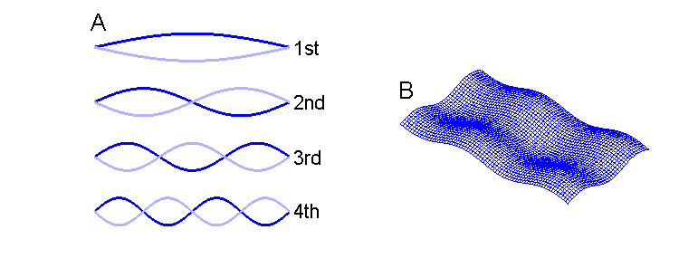
Figure 1.3
A. The first four
modes of vibration of a string. B. A rectangular plate vibrating in the fourth
mode along its length and in the third mode along its width.
Due to these modes, a plucked
guitar string will emit not simply a pure tone corresponding to the resonant
frequency of the whole string, but a mixture that also contains overtones of
twice, three, four, or n times that
resonant frequency. It will, in other words, emit a complex tone—“complex” not
in the sense that it is complicated, but that it is made up of a number of
frequency components, a mixture of harmonically related tones that are layered
on top of each other. The lowest frequency component, the resonant frequency of
the string as a whole, is known as the fundamental frequency, whereas the
frequency components corresponding to the resonance of the half, third, fourth
strings (the second, third and fourth modes of vibration) are called the
“higher harmonics.” The nomenclature of harmonics is a little confusing, in
that some authors will refer to the fundamental frequency as the “zeroth
harmonic,” or F0, and the first harmonic would therefore equal twice
the fundamental frequency, the second harmonic would be three times F0, and the nth harmonic would be n + 1 times F0. Other authors number harmonics differently, and
consider the fundamental to be also the first harmonic, so that the nth harmonic has a frequency of n times F0. We shall adhere
to the second of these conventions, not because it is more sensible, but
because it seems a little more common.
Thus, although many physical
objects such as the strings on an instrument, bells, or xylophone bars
typically emit complex tones made up of many harmonics, these harmonics are not
necessarily present in equal amounts. How strongly a particular harmonic is
represented in the mix of complex tone depends on several factors. One of these
factors is the so-called initial condition. In the case of a guitar string, the
initial condition refers to how, and where, the string is plucked. If you pull
a guitar string exactly in the middle before you let it go, the fundamental
first mode of vibration is strongly excited, because we have delivered a large
initial deflection just at the first mode’s “belly.” However, vibrations in the
second mode vibrate around the center. The center of the string is said to be a
node in this mode of vibration, and vibrations on either side of the node are
“out of phase” (in opposite direction); that is, as the left side swings down
the right side swings up.
To excite the second mode we need
to deflect the string asymmetrically relative to the midpoint. The initial
condition of plucking the string exactly in the middle does not meet this
requirement, as either side of the midpoint is pulled and then released in
synchrony, so the second mode will not be excited. The fourth and sixth modes,
or any other even modes will not be excited either, for the same reason. In
fact, plucking the string exactly in the middle excites only the odd modes of
vibration, and it excites the first mode more strongly than progressively
higher odd modes. Consequently, a guitar string plucked in the middle will emit
a sound with lots of energy at the fundamental, decreasing amounts of energy at
the third, fifth, seventh, … harmonics, and no energy at all at the second,
fourth, sixth… harmonics. If, however, a guitar string is plucked somewhere
near one of the ends, then even modes may be excited, and higher harmonics
become more pronounced relative to the fundamental. In this way, a skilled
guitarist can change the timbre of the sound and make it sound “brighter” or
“sharper.”
Another factor affecting the modes
of vibration of an object is its geometry. The geometry of a string is very
straightforward; strings are, for all intents and purposes, one-dimensional.
But many objects that emit sounds can have quite complex two- and
three-dimensional shapes. Let us briefly consider a rectangular metal plate,
which is struck. In principle, a plate can vibrate widthwise just as easily as
it can vibrate along its length. It could, for example, vibrate in the third
mode along its length and in the second mode along its width, as is
schematically illustrated in figure 1.2B.
Also, in a metal plate, the stiffness stems not from an externally supplied
tension, as in the guitar string, but from the internal tensile strength of the
material.
Factors like these mean that
three-dimensional objects can have many more modes of vibration than an ideal
string, and not all of these modes are necessarily harmonically related. Thus,
a metal plate of an “awkward” shape might make a rather dissonant, unmelodious
“clink” when struck. Furthermore, whether certain modes are possible can depend
on which points of the plate are fixed, and which are struck. The situation
becomes very complicated very quickly, even for relatively simple structures
such as flat, rectangular plates. For more complicated three-dimensional
structures, like church bells, for example, understanding which modes are
likely to be pronounced and how the interplay of possible modes will affect the
overall sound quality, or timbre is as much an art as a science.
To illustrate these points, figure 1.4 shows the frequency spectra of a
piano note and of the chime of a small church bell. What exactly a frequency
spectrum is is explained in greater detail later, but at this point suffice it
to say that a frequency spectrum tells us how much of a particular sinusoid is
present in a complex sound. Frequency spectra are commonly shown using units of
decibel (dB). Decibels are a logarithmic unit, and they can be a little
confusing, which is why we will soon say more about them.
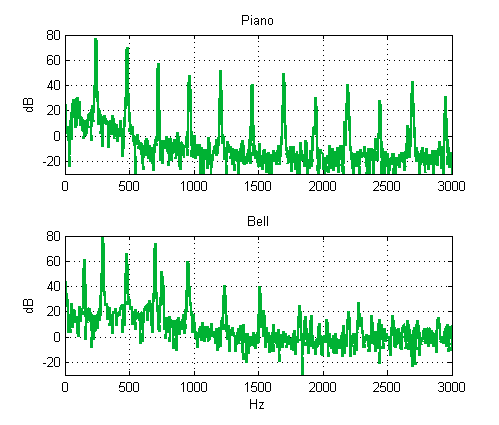
Figure 1.4
Frequency spectra of a
piano and a bell, each playing the note B3 (247 Hz)
To read figure 1.4, all you need to know is that when
the value of the spectrum at one frequency is 20 dB greater than that at
another, the amplitude at that frequency is ten times larger, but if the
difference is 40 dB, then the amplitude is one hundred times greater, and if it
is greater by 60 dB, then it is a whopping one thousand times larger. The piano
and the bell shown in figure 1.4 both play
the musical note B3. (more about musical notes in chapter 3). This
note is associated with a fundamental frequency of 247 Hz, and after our
discussion of modes of vibration, you will not be surprised that the piano note
does indeed contain a lot of 247-Hz vibration, as well as frequencies that are
integer multiples of 247 (namely, 494, 741, 988, 1,235, etc.). In fact,
frequencies that are not multiples of 247 Hz (all the messy bits below 0 dB in figure 1.4) are typically 60 dB, that is, one
thousand times smaller in the piano note than the string’s resonant
frequencies. The spectrum of the bell, however, is more complicated. Again, we
see that a relatively small number of frequencies dominate the spectrum, and
each of these frequency components corresponds to one of the modes of vibration
of the bell. But because the bell has a complex three-dimensional shape, these
modes are not all exact multiples of the 247-Hz fundamental.
Thus real objects do not behave
like an idealized mass spring system, in that they vibrate in numerous modes
and at numerous frequencies, but they also differ from the idealized model in
another important respect. An idealized spring mass system should, once set in
motion, carry on oscillating forever. Luckily, real objects settle down and
stop vibrating after a while. (Imagine the constant din around us if they
didn’t!) Some objects, like guitar strings or bells made of metal or glass, may
continue ringing for several seconds, but vibrations in many other objects,
like pieces of wood or many types of plastic, tend to die down much quicker,
within just a fraction of a second. The reason for this is perhaps obvious. The
movement of the oscillating mass represents a form of kinetic energy, which is
lost to friction of some kind or another, dissipates to heat, or is radiated
off as sound. For objects made of highly springy materials, like steel bells,
almost all the kinetic energy is gradually emitted as sound, and as a
consequence the sound decays relatively slowly and in an exponential fashion.
The reason for this exponential decay is as follows.
The air resistance experienced by
a vibrating piece of metal is proportional to the average velocity of the
vibrating mass. (Anyone who has ever ridden a motorcycle appreciates that air
resistance may appear negligible at low speeds but will become considerable at
higher speeds.) Now, for a vibrating object, the average speed of motion is
proportional to the amplitude of the vibration. If the amplitude declines by
half, but the frequency remains constant, then the vibrating mass has to travel
only half as far on each cycle, but the available time period has remained the
same, so it need move only half as fast. And as the mean velocity declines, so
does the air resistance that provides the breaking force for a further
reduction in velocity. Consequently, some small but constant fraction of the
vibration amplitude is lost on each cycle—the classic conditions for
exponential decay. Vibrating bodies made of less elastic materials may
experience a fair amount of internal friction in addition to the air
resistance, and this creates internal “damping” forces, which are not
necessarily proportional to the amplitude of the vibration. Sounds emitted by
such objects therefore decay much faster, and their decay does not necessarily
have an exponential time course.
By way of example, look at figure 1.5, which shows sound waves from two
musical instruments: one from a wooden castanet, the other from a metal
glockenspiel bar. Note that the time axes for the two sounds do not cover the
same range. The wooden castanet is highly damped, and has a decay constant of
just under 30 ms (i.e., the sound takes 30 ms to decays to 1/e or about 37% of its maximum
amplitude). The metal glockenspiel, in contrast, is hardly damped at all, and
the decay constant of its vibrations is just under 400 ms, roughly twenty times
longer than that of the castanets.
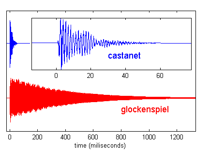
Figure 1.5
A rapidly decaying
(castanet) and a slowly decaying (glockenspiel) sound. The castanet sound is
plotted twice, once on the same time axis as the glockenspiel, and again, in
the inset, with a time axis that zooms in on the first 70 ms.
Thus, the speed and manner with
which a sound decays gives another useful cue to the properties of the material
an object is made of, and few people would have any difficulty using it to
distinguish the sound of a copper bar from that of bar made of silver, even
though some research suggests that our ability to use these cues is not as good
as it perhaps ought to be (Lutfi & Liu, 2007).
We hope the examples in this
section illustratesthat objects in our environment vibrate in complex ways, but
these vibrations nevertheless tell us much about various physical properties of
the object, its weight, its material, its size, and its shape. A vibrating
object pushes and pulls on the air around it, causing vibrations in the air
which propagate as sound (we will look at the propagation of sound in a little
more detail later). The resulting sound is hardly ever a pure tone, but in many
cases it will be made up of a limited number of frequencies, and these are
often harmonically related. The correspondence between emitted frequencies and
physical properties of the sound source is at times ambiguous. Low frequencies,
for example, could be either a sign of high mass or of low tension. Frequency
spectra are therefore not always easy to interpret, and they are not quite as
individual as fingerprints; but they nevertheless convey a lot of information
about the sound source, and it stands to reason that one of the chief tasks of
the auditory system is to unlock this information to help us judge and
recognize objects in our environment. Frequency analysis of an emitted sound is
the first step in this process, and we will return to the idea of the auditory
system as a frequency analyzer in a number of places throughout this book.
1.3 Fourier Analysis and Spectra
In 1822, the French
mathematician Jean Baptiste Joseph Fourier posited that any function whatsoever
can be thought of as consisting of a mixture of sine waves1,
and to this day we refer to the set of sine wave components necessary to make
up some signal as the signal’s Fourier spectrum. It is perhaps surprising that,
when Fourier came up with his idea, he was not studying sounds at all. Instead,
he was trying to calculate the rate at which heat would spread through a cold
metal ring when one end of it was placed by a fire. It may be hard to imagine
that a problem as arcane and prosaic as heat flow around a metal ring would be
sufficiently riveting to command the attention of a personality as big as
Fourier’s, a man who twenty-four years earlier had assisted Napoleon Bonaparte
in his conquests, and had, for a while, been governor of lower Egypt. But
Fourier was an engineer at heart, and at the time, the problem of heat flow
around a ring was regarded as difficult, so he had a crack at it. His reasoning
must have gone something like this: “I have no idea what the solution is, but I
have a hunch that, regardless of what form the solution takes, it must be
possible to express it as a sum of sines and cosines, and once I know that I
can calculate it.” Reportedly, when he first presented this approach to his
colleagues at the
In the context of sounds, however,
which, as we have learned, are often the result of sinusoidal, simple harmonic
motion of spring mass oscillators, Fourier’s approach has a great deal more
immediate appeal. We have seen that there are reasons in physics why we would
expect many sounds to be quite well described as a sum of sinusoidal frequency
components, namely, the various harmonics. Fourier’s bold assertion that it
ought to be possible to describe any
function, and by implication also any variation in air pressure, as a function
of time (i.e., any sound), seems to
offer a nice, unifying approach. The influence of Fourier’s method on the study
of sound and hearing has consequently been enormous, and the invention of
digital computers and efficient algorithms like the fast Fourier transform has
made it part of the standard toolkit for the analysis of sound. Some authors
have even gone so far as to call the ear itself a “biological Fourier
analyzer.” This analogy between Fourier’s mathematics and the workings of the
ear must not be taken too literally though. In fact, the workings of the ear
only vaguely resemble the calculation of a Fourier spectrum, and later we will
introduce better engineering analogies for the function of the ear. Perhaps
this is just as well, because Fourier analysis, albeit mathematically very
elegant, is in many respects also quite unnatural, if not to say downright
weird. And, given how influential Fourier analysis remains to this day, it is
instructive to pause for a moment to point out some aspects of this weirdness.
The mathematical formula of a pure
tone is that of a sinusoid. To be precise, it is A·cos(2π·f·t + φ). The tone oscillates sinusoidally with
amplitude A, and goes through one
full cycle of 2π radians f times in each unit of time t. The period of the pure tone is the time taken for a single cycle,
usually denoted by either a capital T or the Greek letter τ (tau), and is
equal to the inverse of the frequency 1/f.
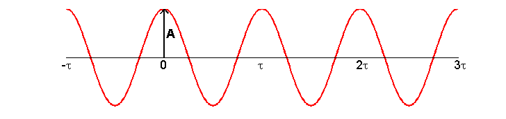
Figure 1.6
A pure tone “in cosine
phase” (remember that cos(0) = 1).
The tone may have had its maximal
amplitude A at time 0, or it may not,
so we allow a “starting phase parameter,” φ,
which we can use to shift the peaks of our sinusoid along the time axis as
required. According to Fourier, we can describe any sound we like by taking a
lot of sine wave equations like this, each with a different frequency f, and if we pick for each f exactly the right amplitude A and the right phase φ, then the sum of these carefully
picked sine waves will add up exactly to our arbitrary sound.
The sets of values of A and φ required to achieve this are known as the sound’s amplitude
spectrum and phase spectrum, respectively. (Amplitude spectra we have encountered
previously in figure 1.4, which
effectively plotted the values of A
for each of the numerous pure tone components making up the sound of a piano or
a bell. Phase spectra, that is, the values of φ for each frequency component, are, as we will see, often
difficult to interpret and are therefore usually not shown.) Note, however,
that, expressed in this mathematically rigorous way, each sine wave component
is defined for all times t. Time 0 is
just an arbitrary reference on my time axis; it is not in any real sense the
time when the sound starts. The Fourier sine wave components making up the
sound have no beginning and no end. They must be thought of as having started
at the beginning of time and continuing, unchanging, with constant amplitude
and total regularity, until the end of time. In that important respect, these
mathematically abstract sine waves could not be more unlike “real” sounds. Most
real sounds have clearly defined onsets, which occur when a sound source
becomes mechanically excited, perhaps because it is struck or rubbed. And real
sounds end when the oscillations of the sound source decay away. When exactly
sounds occur, when they end, and how they change over time are perceptually very
important to us, as these times give rise to perceptual qualities like rhythm,
and let us react quickly to events signaled by particular sounds. Yet when we
express sounds mathematically in terms of a Fourier transform, we have to
express sounds that start and end in terms of sine waves that are going on
forever, which can be rather awkward.
To see how this is done, let us
consider a class of sounds that decay so quickly as to be almost instantaneous.
Examples of this important class of “ultra-short” sounds include the sound of a
pebble bouncing off a rock, or that of a dry twig snapping. These sound sources
are so heavily damped that the oscillations stop before they ever really got
started. Sounds like this are commonly known as “clicks.” The mathematical
idealization of a click, a deflection that lasts only for one single,
infinitesimally short time step, is known as an impulse (or sometimes as a
delta-function). Impulses come in two varieties, positive-going “compression”
clicks (i.e., a very brief upward deflection or increase in sound pressure) or
negative-going “rarefactions” (a transient downward deflection or pressure
decrease).
Because impulses are so short,
they are, in many ways, a totally different type of sound from the complex
tones that we have considered so far. For example, impulses are not suitable
for carrying a melody, as they have no clear musical pitch. Also, thinking of
impulses in terms of sums of sine waves may seem unnatural. After all, a click
is too short to go through numerous oscillations. One could almost say that the
defining characteristic of a click is the predominant absence of sound: A click
is a click only because there is silence both before and immediately after it.
How are we to produce this silence by adding together a number of “always on”
sine waves of the form A·cos(2π·f·t
+ φ)? The way to do this is not exactly intuitively obvious: We have
to take an awful lot of such sine waves (infinitely many, strictly speaking),
all of different frequency f, and get
them to cancel each other out almost everywhere. To see how this works,
consider the top panel of figure 1.7,
which shows ten sine waves of frequencies 1 to 10 Hz superimposed. All have
amplitude 1 and a starting phase of 0.
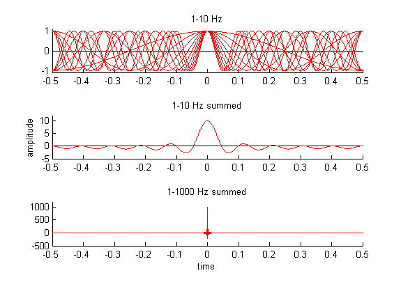
Figure 1.7
Making an impulse from
the superposition of a large number of sine waves.
What would happen if we were to
add all these sine waves together? Well at time t = 0, each has amplitude 1 and they are all in phase, so we would
expect their sum to have amplitude 10 at that point. At times away from zero,
it is harder to guess what the value of the sum would be, as the waves go out
of phase and we therefore have to expect cancellation due to destructive
interference. But for most values of t,
there appear to be as many lines above the x-axis as below, so we might expect
a lot of cancellation, which would make the signal small. The middle panel in figure 1.6 shows what the sum of the ten sine
waves plotted in the top panel actually looks like, and it confirms our
expectations. The amplitudes “pile up” at t
= 0 much more than elsewhere. But we still have some way to go to get
something resembling a real impulse. What if we keep going, and keep adding
higher and higher frequencies? The bottom panel shows what we get if we sum
cosines of frequencies 1 to 1,000. The result is a great deal more clicklike,
and you may begin to suspect that if we just kept going and added infinitely
many cosines of ever-increasing frequency, we would eventually, “in the limit”
as mathematicians like to say, get a true impulse.
Of course, you may have noticed
that, if we approximate a click by summing n
cosines, its amplitude is n, so that,
in the limit, we would end up with an infinitely large but infinitely short
impulse, unless, of course, we scaled each of the infinitely many cosines we
are summing to be infinitely small so that their amplitudes at time 0 could
still add up to something finite. Is this starting to sound a little crazy? It
probably is. “The limit” is a place that evokes great curiosity and wonder in
the born mathematician, but most students who approach sound and hearing from a
biological or psychological perspective may find it a slightly confusing and
disconcerting place. Luckily, we don’t really need to go there.
Real-world clicks are very short,
but not infinitely short. In fact, the digital audio revolution that we have witnessed
over the last few decades was made possible only by the realization that one
can be highly pragmatic and think of time as “quantized”; in other words, we
posit that, for all practical purposes, there is a “shortest time interval” of
interest, know as the “sample interval.” The shortest click or impulse, then,
lasts for exactly one such interval. The advantage of this approach is that it
is possible to think of any sound as consisting of a series of very many such
clicks—some large, some small, some positive, some negative, one following
immediately on another. For human audio applications, it turns out that if we
set this sample period to be less than about 1/40,000 of a second, a sound that
is “sampled” in this manner is, to the human ear, indistinguishable from the
original, continuous-time sound wave.2 Figure 1.8 shows an example of a
sound that is “digitized” in this fashion.
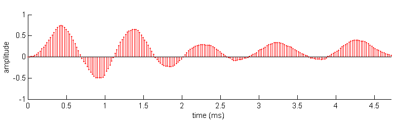
Figure 1.8
One period of the
vowel /a/ digitized at 44.1 kHz.
Each constituent impulse of the
sound can still be thought of as a sum of sine waves (as we have seen in figure 1.7). And if any sound can be thought of
as composed of many impulses, and each impulse in turn can be composed of many
sine waves, then it follows that any sound can be made up of many sine waves.
This is not exactly a formal proof of Fourier’s theorem, but it will do for our
purposes. Of course, to make up some arbitrary sound digitally by fusing
together a very large number of scaled impulses, we must be able to position
each of the constituent impulses very precisely in time. But if one of these impulses
is now to occur at precisely at some time t
= x, rather than at time 0 as in figure 1.6,
then the sine waves making up that particular impulse must now all cancel at
time 0, and pile up at time x. To
achieve this, we have to adjust the “phase term” φ in the equation of each sine wave component of that impulse.
In other words, at time t = x, we
need A·cos(2π·f·t + φ) to
evaluate to A, which means cos(2π·f·x + φ) must equal 1,
and therefore (2π·f·x + φ)
must equal 0. To achieve that, we must set the phase φ of each sine component to be exactly equal to -2π·f·x.
Does this sound a little
complicated and awkward? Well, it is, and it illustrates one of the main
shortcomings of representing sounds in the frequency domain (i.e., as Fourier
spectra): Temporal features of a sound become encoded rather awkwardly in the
“phase spectrum.” A sound with a very simple the time domain description like
“click at time t = 0.3,” can have a
rather complicated frequency domain description such as: “sine wave of
frequency f = 1 with phase φ= -1.88496 plus sine wave of
frequency f = 2 with phase φ= -3.76991 plus sine wave of
frequency f = 3 with phase φ= -5.654867 plus …” and so on.
Perhaps the most interesting and important aspect of the click, namely, that it
occurred at time t = 0.3, is not
immediately obvious in the click’s frequency domain description, and can only
be inferred indirectly from the phases. And if we were to consider a more
complex natural sound, say the rhythm of hoof beats of a galloping horse, then
telling which hoof beat happens when just from looking at the phases of the
Fourier spectrum would become exceedingly difficult. Of course, our ears have
no such difficulty, probably because the frequency analysis they perform
differs in important ways from calculating a Fourier spectrum.
Both natural and artificial sound
analysis systems get around the fact that time disappears in the Fourier
spectrum by working out short-term spectra. The idea here is to divide time
into a series of “time windows” before calculating the spectra. This way, we
can at least say in which time windows a particular acoustic event occurred,
even if it remains difficult to determine the timing of events inside any one
time window. As we shall see in chapter 2, our ears achieve something which
vaguely resembles such a short-term Fourier analysis through a mechanical tuned
filter bank. But to understand the ear’s operation properly, we first must
spend a little time discussing time windows, filters, tuning, and impulse
responses.
1.4 Windowing and Spectrograms
As we have just seen,
the Fourier transform represents a signal (i.e., a sound in the cases that
interest us here) in terms of potentially infinitely many sine waves that last,
in principle, an infinitely long time. But infinitely long is inconveniently
long for most practical purposes. An important special case arises if the sound
we are interested in is periodic, that is, the sound consists of a pattern that
repeats itself over and over. Periodic sounds are, in fact, a hugely important
class of acoustic stimuli, so much so that chapter 3 is almost entirely devoted
to them. We have already seen that sounds that are periodic, at least to a good
approximation, are relatively common in nature. Remember the case of the string
vibrating at its fundamental frequency, plus higher harmonics, which correspond
to the various modes of vibration. The higher harmonics are all multiples of
the fundamental frequency, and the while the fundamental goes through exactly
one cycle, the harmonics will go through exactly two, three, four, … cycles.
The waveform of such periodic sounds is a recurring pattern, and, we can
therefore imagine that for periodic sounds time “goes around in circles,”
because the same thing happens over and over again. To describe such periodic
sounds, instead of a full-fledged Fourier transform with infinitely many
frequencies, we only need a “Fourier series” containing a finite number of
frequencies, namely, the fundamental plus all its harmonics up to the highest
audible frequency. Imagine we record the sound of an instrument playing a very
clean 100-Hz note; the spectrum of any one 10-ms period of that sound would
then be the same as that of the preceding and the following period, as these
are identical, and with modern computers it is easy to calculate this spectrum
using the discrete Fourier transform.
But what is to stop us from taking
any sound, periodic or not, cutting
it into small, say 10-ms wide, “strips” (technically known as time windows),
and then calculating the spectrum for each? Surely, in this manner, we would
arrive at a simple representation of how the distribution of sound frequencies
changes over time. Within any one short time window, our spectral analysis
still poorly represents temporal features, but we can easily see when spectra
change substantially from one window to the next, making it a straightforward
process to localize features in time to within the resolution afforded by a
single time window. In principle, there is no reason why this cannot be done, and
such windowing and short-term Fourier analysis methods are used routinely to
calculate a sound’s spectrogram. In
practice, however, one needs to be aware of a few pitfalls.
One difficulty arises from the
fact that we cannot simply cut a sound into pieces any odd way and expect that
this will not affect the spectrum. This is illustrated in figure 1.9. The top panel of the figure shows a
10-ms snippet of a 1-kHz tone, and its amplitude spectrum. A 1-kHz tone has a
period of 1 ms, and therefore ten cycles of the tone fit exactly into the whole
10–ms-wide time window. A Fourier transform consider this 1-kHz tone as the
tenth harmonic of a 100-Hz tone—100 Hz because the total time window is 10 ms
long, and this duration determines the period of the fundamental frequency
assumed in the transform. The Fourier amplitude spectrum of the 1-kHz tone is
therefore as simple as we might expect of a pure tone snippet: It contains only
a single frequency component. So where is the problem?
Well, the problem arises as soon as
we choose a different temporal window, one in which the window duration is no
longer a multiple of the frequencies we wish to analyze. An example is shown in
the second row of figure 1.9. We are still
dealing with the same pure tone snippet, but we have cut a segment out of it by
imposing a rectangular window on it. The window function is shown in light
gray. It is simply equal to 0 at all the time points we don’t want, and equal
to 1 at all the time points we do want. This rectangular window function is the
mathematical description of an on/off switch. If we multiply the window
function with the sound at each time point then, we get 0 times sound equals 0
during the off period, and 1 times sound equals sound at the on period. You
might think that if you have a 1-kHz pure tone, simply switching it on and off
to select a small segment for frequency analysis, should not alter its
frequency content. You would be wrong.
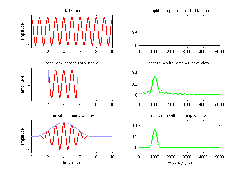
Figure 1.9
The effect of
windowing on the spectrum.
Cast your mind back to figure 1.7, which illustrated the Fourier
transform of a click, and in which we had needed an unseemly large number of
sine waves just to cancel the sound off where we didn’t want it. Something
similar happens when we calculate the Fourier transform of a sine wave snippet
where the period of the sine wave is not a multiple of the entire time window
entered into the Fourier analysis. The abrupt onset and the offset create
discontinuities, that is, “sudden sharp bends” in the waveform, and from the
point of view of a Fourier analysis, discontinuities are broadband signals,
made up of countless frequencies. You might be forgiven for thinking that this
is just a bit of mathematical sophistry, which has little to do with the way
real hearing works, but that is not so. Imagine a nerve cell in your auditory
system, which is highly selective to a particular sound frequency, say a high
frequency of 4,000 Hz or so. Such an auditory neuron should not normally
respond to a 1,000-Hz tone, unless
the 1-kHz tone is switched on or off very suddenly. As shown in the middle panel
of figure 1.9, the onset and offset
discontinuities are manifest as “spectral splatter,” which can extend a long
way up or down in frequency, and are therefore “audible” to our hypothetical
4-kHz cell.
This spectral splatter, which occurs
if we cut a sound wave into arbitrary chunks, can also plague any attempt at
spectrographic analysis. Imagine we want to analyze a so-called
frequency-modulated sound. The whining of a siren that starts low and rises in
pitch might be a good example. At any one moment in time this sound is a type
of complex tone, but the fundamental shifts upward. To estimate the frequency
content at any one time, cutting the sound into short pieces and calculating
the spectrum for each may sound like a good idea, but if we are not careful,
the cutting itself is likely to introduce discontinuities that will make the
sound appear a lot more broadband than it really is. These cutting artifacts
are hard to avoid completely, but some relatively simple tricks help alleviate
them considerably. The most widely used trick is to avoid sharp cutoffs at the
onset and offset of each window. Instead of rectangular windows, one uses
ramped windows, which gently fade the sound on and off. The engineering
mathematics literature contains numerous articles discussing the advantages and
disadvantages of ramps with various shapes.
The bottom panels of figure 1.9 illustrate one popular type, the
Hanning window, named after the mathematician who first proposed it. Comparing
the spectra obtained with the rectangular window and the Hanning window, we see
that the latter has managed to reduce the spectral splatter considerably. The
peak around 1 kHz is perhaps still broader than we would like, given that in
this example we started off with a pure 1-kHz sine, but at least we got rid of
the ripples that extended for several kilohertz up the frequency axis.
Appropriate “windowing” is clearly important if we want to develop techniques
to estimate the frequency content of a sound. But, as we mentioned, the Hanning
window shown here is only one of numerous choices. We could have chosen a
Kaiser window, or a Hamming window, or simply a linear ramp with a relatively
gentle slope. In each case, we would have got slightly different results, but,
and this is the important bit, any of these would have been a considerable
improvement over the sharp onset of the rectangular window. The precise choice
of window function is often a relatively minor detail, as long as the edges of
the window consist of relatively gentle slopes rather than sharp edges.
The really important take-home
message, the one thing you should remember from this section even if you forget
everything else, is this: If we want to be able to resolve individual
frequencies accurately, then we must avoid sharp onset and offset
discontinuities. In other words, we must have sounds (or sound snippets created
with a suitably chosen analysis window) that fade on and off gently—or go on
forever, but that is rarely a practical alternative. Sharp, accurate frequency
resolution requires gentle fade-in and fade-out, which in turn means that the
time windows cannot be very short. This constraint relates to a more general
problem, the so-called time-frequency trade-off.
Let us assume you want to know
exactly when in some ongoing soundscape a frequency component of precisely 500
Hz occurs. Taking on board what we have just said, you record the sound and cut
it into (possibly overlapping) time windows for Fourier analysis, taking care
to ramp each time window on and off gently. If you want the frequency
resolution to be very high, allowing great precision, then the windows have to
be long, and that limits your temporal
precision. Your frequency analysis might be able to tell you that a frequency
very close to 500 Hz occurred somewhere within one of your windows, but because
each window has to be fairly long, and must have “fuzzy,” fading edges in time,
determining exactly when the 500-Hz frequency component started has become
difficult. You could, of course, make your window shorter, giving you greater
temporal resolution. But that would reduce your frequency resolution. This
time-frequency trade-off is illustrated in figure
1.10, which shows a 3-kHz tone windowed with a 10-ms, 5–ms, or 1-ms-wide
Hanning window, along with the corresponding amplitude spectrum.
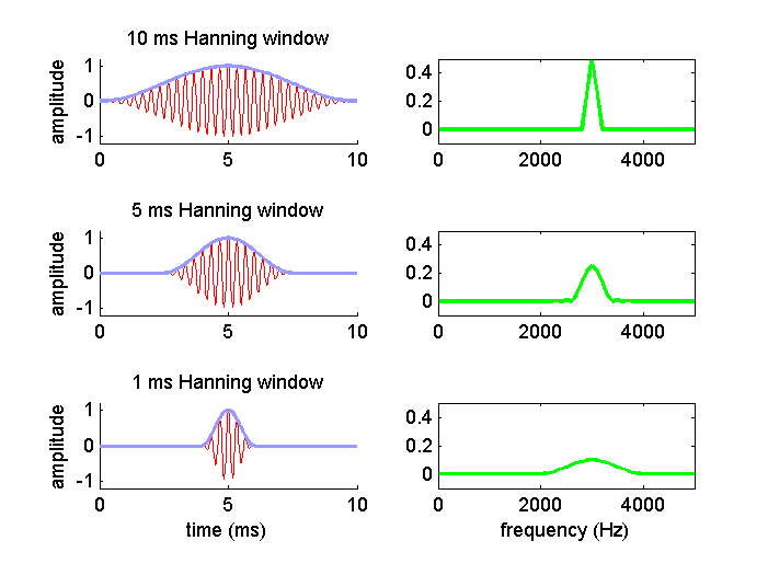
Figure 1.10
The time-frequency
trade-off: Short temporal analysis windows give high temporal precision but
poor spectral resolution.
Clearly, the narrower the window
gets in time, the greater the precision with which we can claim what we are
looking at in figure 1.10 happens at time t = 5 ms, and not before or after; but
the spectral analysis produces a broader and broader peak, so it is
increasingly less accurate to describe the signal as a 3-kHz pure tone rather
than a mixture of frequencies around 3 kHz.
This time-frequency trade-off has
practical consequences when we try to analyze sounds using spectrograms.
Spectrograms, as mentioned earlier, slide a suitable window across a sound wave
and calculate the Fourier spectrum in each window to estimate how the frequency
content changes over time. Figure 1.11
shows this for the castanet sound we had already seen in figure 1.5. The spectrogram on the left was
calculated with a very short, 2.5-ms-wide sliding Hanning window, that on the
right with a much longer, 21-ms-wide window. The left spectrogram shows clearly
that the sound started more or less exactly at time t = 0, but it gives limited frequency (spectral) resolution.
The right spectrogram, in contrast, shows the resonant frequencies of the
castanet in considerably greater detail, but is much fuzzier about when exactly
the sound started.
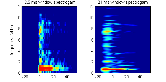
Figure 1.11
Spectrograms of the
castanet sound plotted in figure 1.5,
calculated with either a short (left) or long (right) sliding Hanning window.
The trade-off between time and
frequency resolution is not just a problem for artificial sound analysis
systems. Your ears, too, would ideally like to have both very high temporal
resolution, telling you exactly when a sound occurred, and very high frequency
resolution, giving you a precise spectral fingerprint, which would help you
identify the sound source. Your ears do, however, have one little advantage
over artificial sound analysis systems based on windowed Fourier analysis
spectrograms. They can perform what some signal engineers have come to call
multiresolution analysis.
To get an intuitive understanding
of what this means, let us put aside for the moment the definition of frequency
as being synonymous with sine wave component, and instead return to the
“commonsense” notion of a frequency as a measure of how often something happens
during a given time period. Let us assume we chose a time period (our window)
which is 1 s long, and in that period we counted ten events of interest (these
could be crests of a sound wave, or sand grains falling through an hour glass,
or whatever). We would be justified to argue that, since we observed ten events
per second—not nine, and not eleven—the events happen with a frequency of 10
Hz. However, if we measure frequencies in this way, we would probably be unable
to distinguish 10-Hz frequencies from 10.5- Hz, or even 10.9-Hz frequencies, as
we cannot count half events or other event fractions. The 1-s analysis window
gives us a frequency resolution of about 10% if we wanted to count events
occurring at frequencies of around 10 Hz. But if the events of interest
occurred at a higher rate, say 100 Hz, then the inaccuracy due to our inability
to count fractional events would be only 1%. The precision with which we can
estimate frequencies in a given, fixed time window is greater if the frequency
we are trying to estimate is greater.
We could, of course, do more
sophisticated things than merely count the number of events, perhaps measuring
average time intervals between events for greater accuracy, but that would not
change the fundamental fact that for
accurate frequency estimation, the analysis windows must be large compared to
the period of the signal whose frequency we want to analyze. Consequently,
if we want to achieve a certain level of accuracy in our frequency analysis, we
need very long time windows if the frequencies are likely to be very low, but
we can get away with much shorter time windows if we can expect the frequencies
to be high. In standard spectrogram (short-term Fourier) analysis, we would
have to choose a single time window, which is long enough to be suitable for
the lowest frequencies of interest. But our ears operate like a mechanical filter
bank, and, as we shall see, they can operate using much shorter time windows
when analyzing higher frequency sounds than when analyzing low ones. To get a
proper understanding of how this works, we need to brush up our knowledge of
filters and impulse responses.
1.5 Impulse Responses and Linear Filters
To think of an impulse
as being made up of countless pure-tone frequency components, each of identical
amplitude, as we have seen in figure 1.7,
is somewhat strange, but it can be useful. Let us get back to the idea of a
simple, solid object, like a bell, a piece of cutlery, or a piece of wood,
being struck to produce a sound. In striking the object, we deliver an impulse:
At the moment of impact, there is a very brief pulse of force. And, as we have
seen in sections 1.1 and 1.2, the object responds to this force pulse by
entering into vibrations. In a manner of speaking, when we strike the object we
deliver to it all possible vibration frequencies simultaneously, in one go; the
object responds to this by taking up some of these vibration frequencies, but
it does not vibrate at all frequencies equally. Instead, it vibrates strongly
only at its own resonance frequencies. Consequently, we can think of a struck
bell or tuning fork as a sort of mechanical
frequency filter. The input may contain all frequencies in equal measure,
but only resonant frequencies come out. Frequencies that don’t fit the object’s
mechanical tuning properties do not pass.
We have seen, in figure 1.5, that tuning forks, bells, and other
similar objects are damped. If you strike them to make them vibrate, their
impulse response is an exponentially decaying oscillation. The amplitude of the
oscillation declines more or less rapidly (depending on the damping time
constant), but in theory it should never decay all the way to zero. In
practice, of course, the amplitude of the oscillations will soon become so
small as to be effectively zero, perhaps no larger than random thermal motion
and in any case too small to detect with any conceivable piece of equipment.
Consequently, the physical behavior of these objects can be modeled with great
accuracy by so-called finite impulse
response filters3 (FIRs). Their
impulse responses are said to be finite because their ringing does not carry on
for ever. FIRs are linear systems.
Much scientific discussion has focused on whether, or to what extent, the ear
and the auditory system themselves might usefully be thought of as a set of
either mechanical or neural linear filters. Linearity and nonlinearity are
therefore important notions that recur in later chapters, so we should spend a
moment familiarizing ourselves with these ideas. The defining feature of a
linear system is a proportionality
relationship between input and output.
Let us return to our example of a guitar
string: If you pluck a string twice as hard, it will respond by vibrating with
twice the amplitude, and the sound it emits will be correspondingly louder, but
it will otherwise sound much the same. Because of this proportionality between
input and output, if you were to plot a graph of the force F with which you pluck the string against the amplitude A of the evoked vibration, you would get
a straight line graph, hence the term
“linear.” The graph would be described by the equation A = F∙p, where p is
the proportionality factor which our linear system uses as it converts force
input into vibration amplitude output. As you can hopefully appreciate from
this, the math for linear systems is particularly nice, simple, and familiar,
involving nothing more than elementary-school arithmetic. The corner shop where
you bought sweets after school as a kid was a linear system. If you put twice
as many pennies in, you got twice as many sweets out. Scientists, like most
ordinary people, like to avoid complicated mathematics if they can, and
therefore tend to like linear systems, and are grateful that mother nature
arranged for so many natural laws to follow linear proportionality
relationships. The elastic force exerted by a stretched spring is proportional
to how far the spring is stretched, the current flowing through an ohmic
resistor is proportional to the voltage, the rate at which liquid leaks out of
a hole at the bottom of a barrel is proportional to the size of the hole, the
amplitude of the sound pressure in a sound wave is proportional to the
amplitude of the vibration of the sound source, and so on.
In the case of FIR filters, we can
think of the entire impulse response as a sort of extension of the notion of
proportional scaling in a way that is worth considering a little further. If I
measure the impulse response (i.e., the ping) that a glass of water makes when
I tap it lightly with a spoon, I can predict quite easily and accurately what
sound it will make if I hit it again, only 30% harder. It will produce very
much the same impulse response, only scaled up by 30%. There is an important
caveat, however: Most things in nature
are only approximately linear, over a
limited range of inputs. Strike
the same water glass very hard with a hammer, and instead of getting a greatly
scaled up but otherwise identical version of the previous ping impulse
response, you are likely to get a rather different, crunch and shatter sort of
sound, possibly with a bit of a splashing mixed in if the glass wasn’t empty.
Nevertheless, over a reasonably wide range of inputs, and to a pretty good
precision, we can think of a water glass in front of us as a linear system.
Therefore, to a good first-order approximation, if I know the glass’ impulse
response, I know all there is to know about the glass, at least as far as our
ears are concerned.
The impulse response will allow me
to predict what the glass will sound like in many different situations, not
just if it is struck with a spoon, but also, for example, if it was rubbed with
the bow of a violin, or hit by hail. To see how that works, look at figure 1.12, which schematically illustrates
impulses and impulse responses. The middle panels show a “typical” impulse
response of a resonant object, that is, an exponentially decaying oscillation.
To keep the figure easy to read, we chose a very short impulse response (of a
heavily damped object) and show the inputs, impulse response, and the output as
discrete, digitized, or sampled signals, just as in figure 1.8.
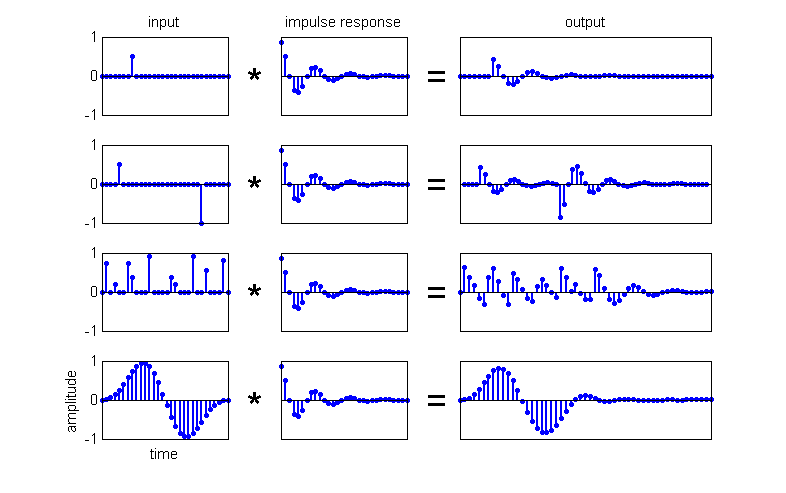
Figure 1.12
Outputs (right panels)
that result when a finite impulse response filter (middle panels) is excited with
a number of different inputs (left panels).
In the top row of figure 1.12, we see what happens when we deliver
a small, slightly delayed impulse to that filter (say a gentle tap with a spoon
on the side of a glass). After our recent discussion of impulse responses and
linearity, you should not find it surprising that the “output,” the evoked
vibration pattern, is simply a scaled, delayed copy of the impulse response
function. In the second row, we deliver two impulses to the same object (we
strike it twice in succession), but the second impulse, which happens after a
slightly larger delay, is delivered from the other side, that is, the force is
delivered in a negative direction. The output is simply a superposition of two impulse responses, each scaled and delayed
appropriately, the second being “turned upside-down” because it is scaled by a
negative number (representing a force acting in the opposite direction). This
should be fairly intuitive: Hit a little bell twice in quick succession, and
you get two pings, the second following, and possibly overlapping with, the
first.
In the second row example, the
delay between the two pulses is long enough for the first impulse response to
die down to almost nothing before the second response starts, and it is easy to
recognize the output as a superposition of scaled and delayed-impulse
responses. But impulses may, of course, come thick and fast, causing impulse
responses to overlap substantially in the resulting superposition, as in the
example in the third row. This shows what might happen if the filter is excited
by a form of “shot noise,” like a series of hailstones of different weights,
raining down on a bell at rapid but random intervals. Although it is no longer
immediately obvious, the output is still simply a superposition of lots of
copies of the impulse response, each scaled and delayed appropriately according
to each impulse in the input. You may notice that, in this example, the output
looks fairly periodic, with positive and negative values alternating every
eight samples or so, even though the input is rather random (noisy) and has no
obvious periodicity at eight samples. The periodicity of the output does, of
course, reflect the fact that the impulse response, a damped sine wave with a
period of eight, is itself strongly periodic. Put differently, since the period
of of the output is eight samples long, this FIR filter has a resonant
frequency which is eight times slower than (i.e. one-eighth of) the sample
frequency. If we were to excite such an FIR filter with two impulses spaced
four samples apart, then the output, the superposition of two copies of the
impulse response starting four samples apart, would be subject to destructive
interference, the peaks in the second impulse response are canceled to some
extent by the troughs in the first, which reduces the overall output.
If, however, the input contains
two impulses exactly eight samples apart, then the output would benefit from
constructive interference as the two copies of the impulse response are
superimposed with peak aligned with peak. If the input contains impulses at
various, random intervals, as in the third row of figure 1.12, then the constructive interference
will act to amplify the effect of impulses that happen to be eight samples
apart, while destructive interference will cancel out the effect of features in
the input that are four samples apart; in this manner, the filter selects out
intervals that match its own resonant frequency. Thus, hailstones raining down
on a concrete floor (which lacks a clear resonance frequency) will sound like
noise, whereas the same hailstones raining down on a bell will produce a
ringing sound at the bell’s resonant frequency. The bell selectively amplifies
(filters) its own resonant frequencies out of the frequency mixture present in
the hailstorm input.
In the fourth row of figure 1.12, we consider one final important
case. Here, instead of delivering a series of isolated impulses to the filter,
we give it a sine wave cycle as input. This is a bit like, instead of striking
a water glass with a spoon, we were to push a vibrating tuning fork against it.
The onset and offset of the sine wave were smoothed off with a Hanning window.
The frequency of the sine wave of the input (one-twentieth of the sample rate)
is quite a bit slower than the resonant frequency of the filter (one-eighth of
the sample rate). What is hopefully quite obvious is that the output is again a
sine whose frequency closely matches that of the input.
This illustrates a very important
property of linear systems. Linear filters cannot introduce new frequency
components; they can only scale each frequency component of the input up or
down, and change its phase by introducing delays. Linear systems are therefore
said to be sine wave in—sine wave out. Conversely, if we observe that a
particular system responds to sine inputs with sine outputs that match the
input frequency, then we would take that as an indication that the system is
linear. And this holds true even if the input is a mixture of several sine
waves. In that case, the output of the linear filter will also be a frequency
mixture, and the relative amplitudes of the various frequency components may
have changed dramatically, but there will be no components at frequencies that
were not present in the input. (Nonlinear filters, in contrast, will quite commonly
introduce frequencies into the output signal that weren’t there in the input!)
Because we had ramped the sine
wave input on and off gently with a Hamming window, the frequency content of
this sine cycle is narrow, and contains very little energy at frequencies
besides one-twentieth of the sample rate. This input therefore cannot excite
the resonant frequency of the linear filter, and, unlike in the hailstones
example in the third row, oscillations with a period of eight samples are not
apparent in the output. The impulse response of the filter itself, however, has
a very sharp onset, and this sharp onset makes its frequency response somewhat
broadband. The input frequency of one-twentieth of the sample rate can
therefore pass through the filter, but it does lose some of its amplitude since
it poorly matches the filter’s resonant frequency. If the impulse response of
the filter had a gentler onset, its frequency response might well be narrower,
and it would attenuate (i.e., reduce the amplitude of) frequencies that are
further from its own resonant frequency more strongly.
In fact, filters with suitably
chosen impulse responses can become quite highly selective for particular
frequencies. We illustrate this in figure 1.13,
which shows what happens when a frequency-modulated signal, a so-called FM
sweep, is filtered through a so-called gamma-tone filter. A gamma-tone is
simply a sinusoid that is windowed (i.e., ramped on and off) with a gamma
function. The only thing we need to know about gamma functions for the purposes
of this book is that they can take the shape of a type of skewed bell, with a
fairly gentle rise and an even gentler decay. Gamma-tone filters are of some
interest to hearing researchers because, as we will see in chapter 2, suitably
chosen gamma-tone filters may provide a quite reasonable first-order
approximation to the mechanical filtering with which the cochlea of your inner
ear analyzes sound. So, if we filter a signal like an FM sweep with a
gamma-tone filter, in a manner of speaking, we see the sound through the eyes
of a point on the basilar membrane of your inner ear (more about that in the
next chapter, and apologies for the mixed metaphor).
When we say the input to the
filter is frequency modulated, we simply mean that its frequency changes over
time. In the example shown in the top panel of figure
1.13, the frequency starts off low but then increases. We made the
signal in this example by computer, but you might encounter such frequency
modulation in real-world sounds, for example, if you plucked the string on a
guitar and then, while the string is still vibrating, either run your finger
down the string along the fret board, making the vibrating part of the string
effectively shorter, or if wind up the tension on the string, increasing its
effective stiffness.
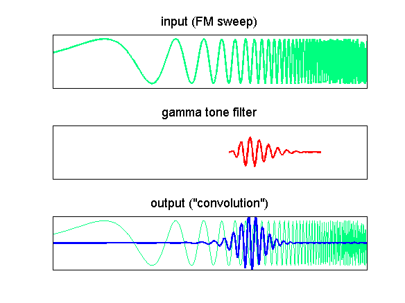
Figure 1.13
An FM sweep filtered
by a gamma-tone filter.
When we compare the gamma-tone
filter in figure 1.13 with the wave-form
of the FM sweep, it should be reasonably obvious that the resonant frequency of
the gamma-tone filter matches the frequency of the FM sweep in some places, but
not in others. In fact, the match between these frequencies starts off and ends
up very poor (the frequency of the FM sweep is initially far too low and
eventually far too high), but somewhere just over halfway through the frequency
of the FM sweep matches that of the filter rather well. And because the
gamma-tone is gently ramped on and off, we expect its frequency bandwidth to be
quite narrow, so as the FM sweep is filtered through the gamma-tone filter, we
expect to see very little in the output at times where the frequencies do not
match. These expectations are fully borne out in the third panel of figure 1.13, which shows the output of the
gamma-tone filter, plotted as a thick black line superimposed on the original
FM sweep input plotted in gray. Frequencies other than those that match the
filter’s resonance characteristics are strongly suppressed.
It is not difficult to imagine
that, if we had a whole series of such gamma-tone filters, each tuned to a
slightly different frequency and arranged in order, we could use the resulting
gamma-tone filter bank to carry out a detailed frequency analysis of incoming
sounds and calculate something very much like a spectrogram on the fly simply
by passing the sounds through all the filters in parallel as they come in. As
it happens, we are all equipped with such filter banks. We call them “ears,”
and we will look at their functional organization in greater detail in the next
chapter. But first we need to add a few brief technical notes to conclude this
section, and we shall see how what we have just learned about filters and
impulse responses can help us understand voices. We also need to say a few
things about the propagation of sound waves through air.
First, the technical notes.
Calculating the output of an FIR filter by superimposing a series of scaled and
delayed copies of the impulse response is often referred to as calculating the
convolution of the input and the impulse responses. Computing convolutions is
sometimes also referred to as convolving. If you look up “convolution,” you
will most likely be offered a simple mathematical formula by way of definition,
something along the lines of “the convolution (f * g)(t) of input f with
impulse response g equals Σ(g(t - τ) ∙ f(τ))
over all τ.” This is really nothing but mathematical shorthand for the
process we have described graphically in figure
1.12. The g(t - τ) bit
simply means we take copies of the impulse response, each delayed by a
different delay τ (tau), and we then scale each of these delayed copies by
the value of the input that corresponds to that delay [that’s the “∙ f(τ)” bit], and then
superimpose all these scaled and delayed copies on top of one another, that is,
we sum them all up (that’s what the “Σ
over all τ” means).
One thing that might be worth
mentioning in passing is that convolutions are commutative, meaning that if we
convolve a waveform f with another
waveform g, it does not matter which
is the input and which is the impulse response. They are interchangeable and
swapping them around would give us the same result: (f * g)(t) = (g * f)(t).
Another thing worth mentioning is
that making computers calculate convolutions is quite straightforward, and
given that so many real-world phenomena can be quite adequately approximated by
a linear system and therefore described by impulse responses, convolution by
computer allows us to simulate all sorts of phenomena or situations. Suppose,
for example, you wanted to produce a radio crime drama, and it so happens that,
according to the scriptwriter, the story line absolutely must culminate in a
satanic mass that quickly degenerates into a violent shootout, all taking place
right around the altar of the highly reverberant acoustic environment of
Well, acoustically speaking,
Or imagine you wanted to make an
electronic instrument, a keyboard that can simulate sounds of other instruments
including the violin. You could, of course, simply record all sorts of notes
played on the violin and, when the musician presses the key on the keyboard,
the keyboard retrieves the corresponding note from memory and plays it. The
problem with that is that you do not know in advance for how long the musician
might want to hold the key. If you rub the bow of a violin across a string it
pulls the string along a little, then the string jumps, then it gets pulled
along some more, then it jumps again a little, and so on, producing a very
rapid and somewhat irregular saw-tooth force input pattern. Such a saw-tooth
pattern would not be difficult to create by computer on the fly, and it can
then be convolved with the strings’ impulse responses, that is, sounds of the
strings when they were plucked, to simulate the sound of bowed strings. Of
course, in this way you could also simulate what it would sound like if objects
were “bowed” that one cannot normally bow, but for which one can either record
or simulate impulse responses: church bells, plastic bottles, pieces of
furniture, and so on. Convolution is thus a surprisingly versatile little tool
for the computer literate who enjoy being scientifically or artistically
creative.
1.6 Voices
An important class of sounds,
which is much easier to understand now that we have discussed impulse responses
and convolutions, is voices. Given their central role in spoken words, song,
and animal communication, voices are a particularly important class of sounds,
and like many other sounds that we have discussed already, voices too are a
kind of pulse-resonance sound. When humans or other mammals vocalize, they
tighten a pair of skin flaps known as vocal folds across their airways (the
larynx), and then exhale to push air through the closed vocal folds. The vocal
folds respond by snapping open and shut repeatedly in quick succession,
producing a series of rapid clicks known as “glottal pulses.” These glottal
pulses then “ring” through a series of resonant cavities, the vocal tract ,
which includes the throat, the mouth, and the nasal sinuses. (Look for a video
showing human vocal folds in action on the book’s web site <flag>). When
we speak, we thus effectively convolve a glottal pulse train with the resonant
filter provided by our vocal tract, and we can change our voice, in rather
different and interesting ways, either by changing the glottal pulse train or
by changing the vocal tract.
First, let us consider the glottal
pulse train, and let us assume for simplicity that we can approximate this as a
series of “proper” impulses at very regular intervals. Recall from figure 1.7 that any impulse can be thought of as
a superposition of infinitely many sine waves, all of the same amplitude but
different frequency, and with their phases arranged in such a way that they all
come into phase at the time of the impulse but at no other time. What happens
with all these sine waves if we deal not with one click, but with a series of
clicks, spaced at regular intervals?
Well, each click is effectively
its own manifestations of infinitely many sine waves, but if we have more than
one click, the sine waves of the individual clicks in the click train will
start to interfere, and that interference can be constructive or destructive.
In fact, the sine components of the two clicks will have the same phase if the
click interval happens to be an integer (whole number) multiple of the sine
wave period, in other words if exactly one or two or three or n periods of the sine wave fit between
the clicks. The top panel of figure 1.14 may help you appreciate that fact. Since these sine waves are present,
and in phase, in all clicks of a regular click train of a fixed interval, these
sine waves will interfere constructively and be prominent in the spectrum of
the click train. However, if the click interval is 1/2, or 3/2, or 5/2,… of the
sine period, then the sine components from each click will be exactly out of
phase, as is shown in the bottom panel of figure
1.14, and the sine components cancel out.
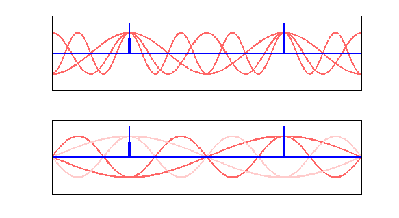
Figure 1.14
Sine components of
click trains interfere constructively when the sine period is an integer
multiple of the click interval, but not otherwise.
The upshot of this is that a
regular, periodic click train is effectively a type of sound that we had
already encountered in section 1.2, namely, a type of complex tone, made up of
a fundamental frequency and an infinite number of higher harmonics, all of
equal amplitude. The periods of the harmonics are equal to 1/1, 1/2, 1/3, … 1/n of the click interval, and their
frequencies are accordingly multiples of the fundamental. Consequently, the
closer the clicks are spaced in time, the wider apart the harmonics are in
frequency.
All of this applies to glottal
pulse trains, and we should therefore not be surprised that the spectrogram of
voiced speech sounds exhibits many pronounced harmonics, reaching up to rather
high frequencies. But these glottal pulse trains then travel through the
resonators of the vocal tract. Because the resonant cavities of the throat,
mouth, and nose are linear filters, they will not introduce any new
frequencies, but they will raise the amplitude of some of the harmonics and suppress
others.
With this in mind, consider the
spectrogram of the vowel /a/, spoken by a male adult, shown in figure 1.15. The spectrogram was generated with
a long time window, to resolve the harmonics created by the glottal pulse
train, and the harmonics are clearly visible as spectral lines, every 120 Hz or
so. However, some of the harmonics are much more pronounced than others. The
harmonics near 700 to 1,200 Hz are particularly intense, while those between
1,400 and 2,000 Hz are markedly weaker, and then we see another peak at around
2,500 Hz, and another at around 3,500 Hz. To a first approximation, we can
think of each of the resonators of the vocal tract as a band pass filter with a
single resonant frequency. These resonant frequencies are known as “formants,”
and those harmonics that lie close to the formant frequencies will be scaled up
relative to the others, which leads to the peaks we have just observed.
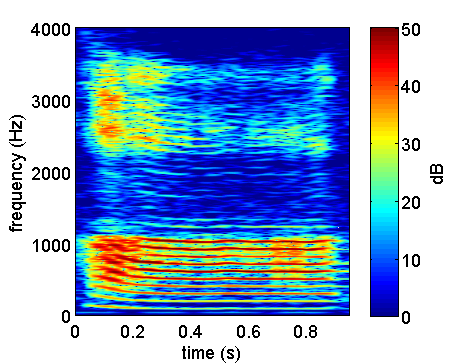
Figure 1.15
Spectrogram of the
vowel “a.”
One important feature of our voice
is that it gives us independent control of the harmonic and the formant
frequencies. We change the harmonic frequencies by putting more or less tension
on our vocal folds. The higher the tension, the faster the glottal pulse train,
which leads to a higher the fundamental frequency and more widely spaced
harmonics, and the voice is perceived as higher pitched. The formant
frequencies we control by moving various parts of our vocal tract, which are
commonly referred to as “articulators,” and include the lips, jaws, tongue, and
soft palate. Moving the articulators changes the size and shape of the
resonance cavities in the vocal tract, which in turn changes their resonant
frequencies, that is, the formants.
This does not affect the pitch of
the speech sound, but its timbre, and therefore its type may change quite
dramatically, for example, if we change between /o/- and /a/-like vowels simply
by widening the opening of our lips and jaw. Thus, we control which vowel we
produce by changing the formant frequencies, and we control the pitch at which
we speak or sing a vowel by changing the harmonic frequencies. This can be seen
quite clearly in figure 1.16, which shows
spectrograms of the words “hot,” “hat,” “hit,” and “head,” spoken by different
native speakers of British English, one with a high–pitched, child-like voice
(top row) and then again in a lower-pitched voice of an adult female (bottom
row). A color version of that figure, along with the corresponding sound
recordings, can be found on the “vocalizations and speech” section of the
book’s web site <flag>).
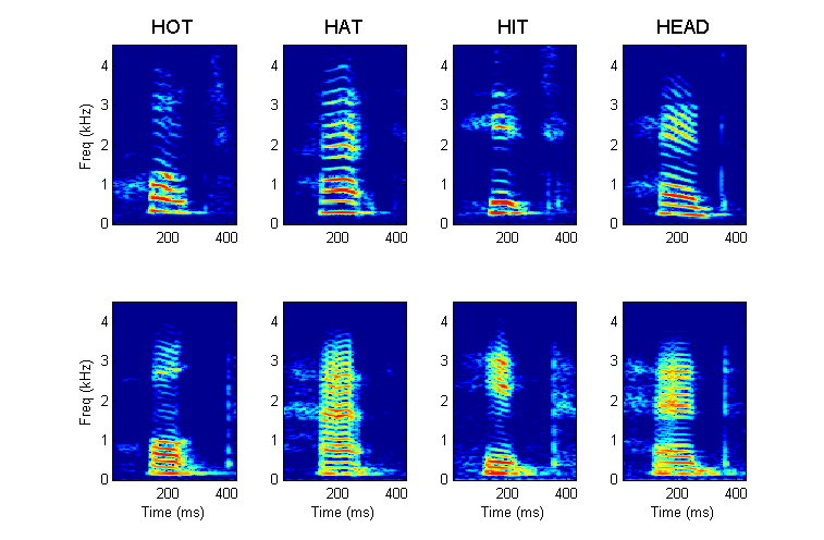
Figure 1.16
Spectrograms of the
words “hot,” “hat,” “hit,” and “head,” spoken in a high-pitched (top row) and a
low-pitched (bottom row) voice.
The vowels in the spoken words are
readily apparent in the “harmonic stacks” that mark the arrival of the glottal
pulse train, and the spacing of the harmonics is clearly much wider in the
high-pitched than in the low-pitched vowels. The fact that, in some of the
sounds, the harmonics aren’t exactly horizontal tells us that the pitch of
these vowels was not perfectly steady (this is particularly noticeable in the
high-pitched “hot” and “head”). Where exactly the formants are in these vowels
is perhaps not quite so readily apparent to the unaided eye. (Formants are, in
fact, easier to see in spectrograms that have short time windows, and hence a
more blurred frequency resolution, but then the harmonics become hard to
appreciate.) But it is nevertheless quite clear that, for example, in the /i/
sounds the harmonics around 500 Hz are very prominent, but there is little
sound energy between 800 and 2000 Hz, until another peak is reached at about
2,300 Hz, and another near 3,000 Hz. In contrast, in the /a/ vowels, the energy
is much more evenly distributed across the frequency range, with peaks perhaps
around 800, 1,800, and 2,500 Hz, while the /o/ sound has a lot of energy at a
few hundred Hertz, up to about 1,100 Hz, then much less until one reaches
another smaller peak at 2,500 Hz.
Of course, there is more to the
words “hot,” “hat,” “hit,” and “head” than merely their vowels. There are also
the consonants “h” at the beginning and
“t” and “d” at the end. Consonants can be subdivided into different classes
depending on a number of criteria. For example, consonants can be “voiced” or
“unvoiced” . If they are voiced, the vocal folds are moving and we would expect
to see harmonics in their spectrogram. The “h” and the “t” in “hot,” “hat,” “hit,”
and “head” are unvoiced, the vocal chords are still. So what generates the
sounds of these unvoiced consonants? Most commonly, unvoiced consonants are
generated when air is squeezed through a narrow opening in the airways,
producing a highly turbulent flow, which sets up random and therefore noisy
vibration patterns in the air.
In speaking the consonant “h,” the
air “rubs” as it squeezes through a narrow opening at the back of the mouth.
Students of phonetics, the science of speech sounds, would therefore describe
this sound as a glottal (i.e., throat produced) fricative (i.e., rubbing
sound), in this manner describing the place and the mode of articulation. The
“t” is also produced by the tongue, but unlike in pronouncing the “h,” the
airway is at first blocked and then the air is released suddenly, producing a
sharp sound onset characteristic of a “plosive” stop consonant. Plosives can
be, for example, “labial,” that is, produced by the lips as in “p” or “b”; or
they can be “laminal-dental,” that is, produced when the tip of the tongue, the
lamina, obstructs and then releases the airflow at the level of the teeth, as
in “t” or “d”; or they can be velar, that is, produced at the back of the
throat when the back of the tongue pushes against the soft palate; or velum ,
as in “k.”
The mouth and throat area contains
numerous highly mobile parts that can be reconfigured in countless different
ways, so the number of possible speech sounds is rather large. (See the
“vocalization and speech” section of the book’s website for links to x-ray
videos showing the human articulators in action <flag >). Cataloguing all
the different speech sounds is a science in itself, known as articulatory
phonetics. We shall not dwell on this any further here, except perhaps to point
out a little detail in figure 1.16, which
you may have already noticed. The “h” fricative at the beginning of each word
is, as we have just described, the result of turbulent airflow, hence noisy,
hence broadband; that is, it should contain a very wide range of frequencies.
But the frequencies of this consonant are subjected to resonances in the vocal
tract just as much as the harmonics in the vowel. And, indeed, if you look
carefully at the place occupied by the “h” sounds in the spectrograms of figure 1.16 (the region just preceding the
vowel), you can see that the “h” sound clearly exhibits formants, but these
aren’t so much the formants of the consonant “h” as the formants of the vowel
that is about to follow! When we pronounce “hot” or “hat,” our vocal tract
already assumes the configuration of the upcoming vowel during the “h,”
imparting the formants of the following vowel onto the preceding consonant.
Consequently, there is, strictly speaking, really no such thing as the sound of
the consonant “h,” because the “h” followed by an “o” has really quite a
different spectrum from that of an “h” that is followed by an “a.”
This sort of influence of the
following speech sound onto the preceding sound is sometimes referred to as
“coarticulation” or “assimilation” in the phonetic sciences, and it is much
more common than you might think. In your personal experience, an “h” is an
“h”; you know how to make it, you know what it sounds like. Recognizing an “h”
is trivially easy for your auditory system, despite the fact that, in reality,
there are many different “h” sounds. This just serves to remind us that there
is a lot more to hearing than merely accurately estimating frequency content,
and for people trying to build artificial speech recognizers, such phenomena as
coarticulation can be a bit of a headache.
1.7 Sound Propagation
So far, we have looked
almost exclusively at vibration patterns in a variety of sound sources.
Developing some insights into how sounds come about in the first place is an
essential, and often neglected, aspect of the auditory sciences. But, of
course, this is only the beginning. We can hear the sound sources in our
environment only if their vibrations are somehow physically coupled to the
vibration-sensitive parts of our ears. Most commonly, this coupling occurs
through the air.
Air is capable of transmitting
sound because it has two essential properties: inert mass and stiffness or
elasticity. You may not think of air as either particularly massive or
particularly elastic, but you probably do know that air does weigh something
(about 1.2 g/L at standard atmospheric pressure), and its elasticity you can
easily verify if you block off the end of a bicycle pump and then push down the
piston. As the air becomes compressed, it will start to push back against the
piston, just as if it were a spring. We can imagine the air that surrounds us
as being made up of small “air masses,” each linked to its neighboring masses
through spring forces that are related to air pressure. This is a useful way of
conceptualizing air, because it can help us develop a clear image of how sound
waves propagate. A medium made of small masses linked by springs will allow
disturbances (e.g., small displacements at one of the edges) to travel through
the medium from one mass to the next in a longitudinal wave pattern. How this
works is illustrated in figure 1.17, as
well as in a little computer animation which you can find on the book’s web
site <flag>.
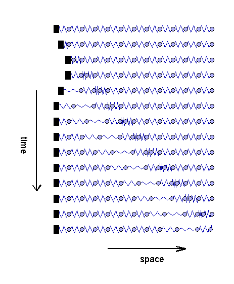
Figure 1.17
A longitudinal wave
propagating through a medium of inert masses coupled via elastic springs. See
the book’s Web site www.auditoryneuroscience.com for an animated version.
Figure
1.17 shows the
output of a computer simulation of a sound source, represented by the black
rectangle to the right, which is in contact with an air column, represented by
a row of air masses (gray circles) linked by springs (zigzag lines). At first
(top row), the source and the air masses are at rest, but then the sound source
briefly lurches a bit to the right, and then returns to its initial position.
The rightward movement compresses the spring that links it to the neighboring
air mass. That, in turn, causes this air mass to be accelerated rightwards, but
because the mass has a small inertia, its movement lags somewhat behind that of
the sound source. As the mass immediately to the right of the sound source
starts moving rightward, it compresses the spring linking it to the next mass
along, which in turn accelerates that mass rightward, and so on and so on. As
the sound source returns to its original position, it will start to stretch the
spring linking it to the neighboring mass, which in time will pull that mass
back to its original position. This stretch also propagates along the air
column; thus, while each air mass is first pushed one way it is then pulled the
other, so that it ends up where it started. There are thus essentially four
phases to the propagating sound wave: first, a compression, followed by a
forward displacement, followed by a rarefaction (or stretch, in our spring
analogy), followed by a backward (return) displacement. Sound waves therefore
consist of displacement waves as well as pressure waves, but the displacement
wave lags behind the pressure wave by a quarter of a cycle, and the final net
displacement of the air is zero. (Sound is not a wind).
To generate figure 1.17, we got a computer to apply Hooke’s
law to work out all the spring forces, and then to use Newton’s second law to
calculate the acceleration of each inert air mass in turn and update the
positions of the masses accordingly at each time step. Figure 1.17 illustrates quite nicely how the
simple interaction of Hooke’s law and Newton’s second law allows for a movement
of a sound source to be translated into a “disturbance” in the local air
pressure (the spring forces), which then propagates through a column of air
away from the source. It is essentially that mechanism which links the surfaces
of all the sound sources in your environment to your eardrum. And in doing so,
it replicates the vibration patterns of the sound sources quite accurately. The
forward movement of the source gave rise to a compression of corresponding
size, while the return to the original position created a corresponding
rarefaction. This simple correspondence is handy, because it means that we can,
to a pretty good first approximation, assume that everything we have learned in
previous sections about the vibration patterns of different types of sound sources
will be faithfully transmitted to the eardrum.
Of course, this phenomenon of
longitudinal propagation of waves is not limited to air. Any material that
possesses inert mass and at least some springlike elasticity is, in principle,
capable of propagating sound waves. Consequently, dolphins can use their lower
jaws to pick up sound waves propagated through water, while certain species of
toads, or even blind mole rats, appear to be able to collect sound waves
conducted through the ground. But different substrates for sound propagation
may be more or less stiff, or more or less heavy, than air, and these
differences will affect the speed at which sound waves travel through that
substrate. We mentioned earlier that the displacement of the first air mass in figure 1.17 lags somewhat behind the
displacement of the sound source itself. The movement of the sound source first
has to compress the spring, and the spring force then has to overcome the
inertia of the first mass. Clearly, if the spring forces are quite large and
the masses only small, then the time lag will not be very great.
Materials with such comparatively
large internal spring forces are said to have a high acoustic impedance. The
acoustic impedance is defined as the amount of pressure (i.e., spring force)
required to achieve a given particle velocity. The speed of sound is high in
materials that have a high acoustic impedance but a low density (essentially
high spring forces and low masses). For air at ambient pressures and
temperature, the speed of sound works out to about 343 m/s (equivalent to 1,235
km/h or 767 mph). The precise value depends on factors such as humidity,
atmospheric pressure, and temperature, because these may affect the mass
density and the elastic modulus (i.e., the springiness) of the air. For water,
which is heavier but also much, much stiffer than air, the speed of sound is
more than four times larger, at about 1,480 m/s (5,329 km/h or 3,320 mph).
In a number of ways, the
longitudinal wave propagation shown in figure
1.17 is, of course, a somewhat oversimplified model of real sound waves.
For example, in our idealized model, sound waves propagate without any loss of
energy over infinite distances. But you know from experience that sounds are
quieter if the sound source is further away. Two factors contribute to this.
The first, and often the less important reason, is that in real physical media,
sound waves tend to dissipate , which simply means that the coordinated motion
of air masses will start to become disorganized and messy, gradually looking
less and less like a coherent sound wave and increasingly like random motion;
that is, the sound will slowly turn into heat. Interestingly, high-frequency
sounds tend to dissipate more easily than low-frequency ones, so that thunder heard
from a great distance will sound like a low rumble, even though the same sound
closer to the source would have been more of a sharp “crack,” with plenty of
high-frequency energy. Similarly, ultrasonic communication and echolocation
sounds such as those used by mice or bats tend to have quite limited ranges. A
mouse would find it very difficult to call out to a mate some twenty yards
away, something that most humans can do with ease.
The second, and usually major factor
contributing to the attenuation (weakening) of sounds with distance stems from
the fact that most sound sources are not linked to just a single column of
spring-linked masses, as in the example in figure
1.17, but are instead surrounded by air. We really should think more in
terms of a three-dimensional lattice of masses with spring forces acting up and
down, forward and backward, as well as left and right. And as we mentioned
earlier, the springs in our model represent air pressure gradients, and you may
recall that pressure will push from the point where the pressure is greater in all directions where pressure is
lower. Consequently, in a three-dimensional substrate, a sound wave that starts
at some point source will propagate outward in a circular fashion in all
directions. You want to imagine a wavefront a bit like that in figure 1.17, but forming a spherical shell that
moves on outward from the source.
Now, this spherical shell of the
propagating sound wave does, of course, get larger and larger as the sound
propagates, just like the skin of a balloon gets larger as we continue to
inflate it. However, all the mechanical energy present in the sound wave was
imparted on it at the beginning, when the sound source accelerated the air
masses in its immediate neighborhood. As the sound wave propagates outward in a
sphere, that initial amount of mechanical energy gets stretched out over a
larger and larger area, much like the skin of a balloon becomes thinner as we
inflate it. If the area becomes larger as we move further away from the sound
source but the energy is constant, then the amount of energy per unit area must
decrease. And since the surface area of a sphere is proportional to the square
of its radius (surface = 4∙π ∙r2),
the sound energy per unit surface area declines at a rate that is inversely
proportional to the square of the distance from the source. This fact is often
referred to as the inverse square law, and it is responsible for the fact that
sound sources normally are less loud as we move further away from them.
Of course, the inverse square law,
strictly speaking, only holds in the “free field,” that is, in places where the
sound wave really can propagate out in a sphere in all directions. If you send
sound waves down a narrow tube with rigid walls, then you end up with a
situation much more like that in figure 1.17,
where you are dealing with just a column of air in which the sound amplitude
should stay constant and not decline with distance. You may think that this is
a severe limitation, because in the real world there are almost always some
surfaces that may be an obstacle to sound propagation, for example, the floor!
However, if you placed a sound source on a rigid floor, then the sound waves
would propagate in hemispheres outwards (i.e., sideways and upward), and the
surface area of a hemisphere is still proportional to the square of its radius
(the surface is simple half of 4πr2,
hence still proportional to r2),
so the inverse square law would still apply.
If, however, we lived in a world
with four spatial dimensions, then sound energy would drop off as a function of
1/r3—which would be known
as the inverse cube law—and because sound waves would have more directions in
which they must spread out, their amplitudes would decrease much faster with
distance, and communicating with sound over appreciable distances would require
very powerful sound sources. Of course, we cannot go into a world of four
spatial dimensions to do the experiment, but we can send sound down
“effectively one-dimensional” (i.e., long but thin) tubes. If we do this, then
the sound amplitude should decrease as a function of 1/r0 = 1, that is, not at all, and indeed people in the
1800s were able to use long tubes with funnels on either end to transmit
voices, for example, from the command bridge to the lower decks of a large
ship.
Thus, the inverse square law does
not apply for sounds traveling in confined spaces, and substantial deviations
from the inverse square law are to be expected also in many modern indoor
environments that, albeit three-dimensional, nevertheless contain many
sound-reflecting surfaces, including walls and ceilings, which will cause the
sound waves to bounce back and forth, creating a complex pattern of overlapping
echoes known as reverberations . In such reverberant environments, the sound
that travels directly from the source to the receiver, will obey the inverse
square law, but reflected sound waves will soon add to this original sound.
1.8 Sound Intensity
From our previous
discussion of propagating sound waves, you probably appreciate the dual nature
of sound: A small displacement of air causes a local change in pressure, which
in turn causes a displacement, and so on. But if we wanted to measure how large
a sound is, should we concern ourselves with the amplitude of the displacement,
or its velocity, or the amplitude of the pressure change, or all three? Well,
the displacement and the pressure are linked by linear laws of motion, so if we
know one, we ought to be able to work out the other. The microphones used to
measure sounds typically translate pressure into voltage, making it possible to
read the change of pressure over time directly off an oscilloscope screen.
Consequently, acoustical measures of sound amplitude usually concern themselves
with the sound pressure only. And you might think that, accordingly, the
appropriate thing to do would be to report sound amplitudes simply in units of
pressure, that is, force per unit area. While this is essentially correct,
matters are, unfortunately, a little more complicated.
The first complication we have to
deal with is that it is in the very nature of sounds that the sound pressure
always changes, which is very inconvenient if we want to come up with a single
number to describe the intensity of a sound. We could, of course, simply use
the largest (peak) pressure in our sound
wave and report that. Peak measurements like that are sometimes used, and are
perfectly fine if the sound we try to characterize is a pure sinusoid, for
example, because we can infer all the other amplitudes if we know the peak
amplitude. But for other types of sound, peak amplitude measures can be quite
inappropriate. Consider, for example, two click trains, each made up of
identical brief clicks; but in the first click train the interval between
clicks is long, and in the second it is much shorter. Because the clicks are
the same in each train, the peak amplitudes for the two trains are identical,
but the click train with the longer inter-click intervals contains longer
silent periods, and it would not be unreasonable to think it therefore has, in
an manner of speaking, less sound in it than the more rapid click train.
As this example illustrates, it is
often more appropriate to use measures that somehow average the sound pressure
over time. But because sounds are normally made up of alternating compressions
and rarefactions (positive and negative pressures), our averaging operation
must avoid canceling positive against negative pressure values. The way this is
most commonly done is to calculate the root-mean-square (RMS) pressure of the sound wave.
As the name implies, RMS values
are calculated by first squaring the pressure at each moment in time, then
averaging the squared values, and finally taking the square root. Because the
square of a negative value is positive, rarefactions of the air are not
canceled against compressions when RMS values are calculated. For sine waves,
the RMS value should work out as 1 / √ 2 (ca 70.71%) of the peak value, but that is true only if the averaging
for the RMS value is done over a time period that contains a whole number of
half-cycles of the sine wave. In general, the values obtained with any
averaging procedure to some extent will be sensitive to the choice of time
window over which the averaging is done, and the choice of the most appropriate
time window will depend on the particular situation and may not always be
obvious.
Another factor that can cause
great confusion among newcomers to the study of sound (and sometimes even among
experts) is that even RMS sound pressure values are almost never reported in
units of pressure, like in pascals (newtons per square meter) or in bars, but
are instead normally reported in bels, or more commonly in tenths of bels,
known as decibels (dB) . Bels are in many ways a very different beast from the
units of measurement that we are most familiar with, like the meter, or the
kilogram, or the second. For starters, unlike these other units, a bel is a logarithmic unit. What is that supposed
to mean?
Well, if I give, for example, the
length of a corridor as 7.5 m, then I effectively say that it is 7.5 times as long as a well-defined standard
reference length known as a meter. If, however, I report an RMS sound pressure
as 4 bels (or 40 dB), I’m saying that it is 4 orders of magnitude (i.e., 4 powers of 10 = 104 = 10,000
times) larger than some standard reference pressure. Many newcomers to
acoustics will find this orders of magnitude thinking unfamiliar and at times a
little inconvenient. For example, if I add a 20-kg weight to a 40-kg weight, I
get a total weight of 60 kg. But if I add, in phase, a 1-kHz pure tone with an
RMS sound pressure amplitude of 20 dB to another 1-kHz pure tone with an
amplitude of 40 dB, then I do not end up with a tone with a 60-dB amplitude.
Instead, the resulting sound pressure would be log10(104 +
102) = 4.00432 bels, that is, 40.0432 dB. The weaker of the two
sounds, having an amplitude 2 orders of magnitude (i.e., 100 times) smaller
than the larger one, has added, in terms of orders of magnitude, almost nothing
to the larger sound.
Because decibels, unlike weights
or lengths or money, work on a logarithmic scale, adding decibels is a lot more
like multiplying sound amplitudes than adding to them, and that takes some
getting used to. But the logarithmic nature of decibels is not their only
source of potential confusion. Another stems from the fact that decibels are
used to express all sorts of logarithmic ratios, not just ratios of RMS sound
pressure amplitudes. Unlike meters, which can only be used to measure lengths,
and always compare these lengths to a uniquely and unambiguously defined
standard length, for decibels there is no uniquely defined type of measurement,
nor is there a unique, universally accepted standard reference values. Decibel
values simply make an order of magnitude comparison between any two quantities,
and one must try to be clear in one’s mind about what is being compared to
what.
Decibel values need not relate to
sound at all. To say that the sun is about 25.8 dB (i.e., 102.58, or
roughly 380 times) further away from the earth than the moon would perhaps be a
little unusual, but entirely correct. But surely, at least in the context of
sound, can’t we safely assume that any decibels we encounter will refer to
sound pressure? Well, no. Sometimes they will refer to the RMS pressure,
sometimes to peak pressure, but more commonly, acoustical measurements in
decibels will refer to the intensity
or the level of a sound. In a context
of acoustics, the words “level” and “intensity” can be used interchangeably,
and an intensity or level stated in decibels is used, in effect, to compare the
power (i.e., the energy per unit
time) per unit area delivered by each of the two sound waves.
Fortunately, there is a rather
simple relationship between the energy of a sound and its RMS sound pressure
amplitude, so everything we learned so far about pressure amplitudes will still
be useful. You may remember from high school physics that the kinetic energy of
a moving heavy object is given by E = mv2,
that is, the kinetic energy is proportional to the square of the velocity. This
also holds for the kinetic energy of our notional lumps of air, which we had
encountered in figure 1.17 and which that
take part in a longitudinal wave motion to propagate sound. Now, the average
velocity of these lumps of air is proportional to the RMS sound amplitude, so
the energy levels of the sound are proportional to the square of the amplitude. Consequently, if I wanted to work out the
intensity y of a particular sound
with RMS pressure x in decibel
relative to that of another known reference sound whose RMS pressure is xref, then I would do this
using the formula
y (dB) = 10 ∙ log10(x2 / xref2) = 20 ∙ log10(x/xref)
(The factor of 10
arises because there are 10 dB in a bel. And because log(a2) = 2∙log(a), we can bring the squares in the
fraction forward and turn the factor 10 into a factor 20).
You might be forgiven for
wondering whether this is not all a bit overcomplicated. If I can use a
microphone to measure sound pressure directly, then why should I go to the
trouble of first expressing the observed pressure amplitudes as multiples of
some reference, then calculating the log to base 10 of that fraction, then
finally multiply by20 to work out a decibel sound intensity value. Would it not
be much easier and potentially less confusing to simply state the observed
sound pressures amplitudes directly in pascals? After all, our familiar, linear
units like the meter and the newton and the gram, for which 4 + 2 = 6, and not
4.00432, have much to commend themselves. So why have the seemingly more
awkward and confusing logarithmic measures in bels and decibels ever caught on?
Well, it turns out that, for the
purposes of studying auditory perception, the orders of magnitude thinking that
comes with logarithmic units is actually rather appropriate, for a number of
reasons. For starters, the range of sound pressure levels that our ears can
respond to is quite simply enormous. Hundreds of millions of years of evolution
during which you get eaten if you can’t hear the hungry predators try to creep
up on you have equipped us with ears that are simply staggeringly sensitive.
The faintest sound wave that a normal, young healthy human can just about hear
has an RMS sound pressure of roughly 20 micropascal (μPa), that is, 20
millionth of a newton per square meter. That is approximately 10 million times
less than the pressure of a penny resting on your fingertip! Because an
amplitude 20 μPa is close to the absolute threshold of human hearing, it
is commonly used as a reference for sound intensity calculations. Sound levels
expressed in decibels relative to 20 μPa are usually abbreviated as dB SPL, short for sound pressure level.
The sound level of the quietest
audible sounds would therefore be around 0 dB SPL. (These almost inaudibly
quiet sounds have an amplitude approximately equal to that of the reference of
20 μPa, so the fraction x/xref
in the formula above would work out to about 1, and the log of 1 is 0.) But if
you listen, for example, to very loud rock music, then you might expose your
ears to sound levels as high as 120 dB SPL. In other words, the sound energy
levels in these very loud sounds are twelve orders of
magnitude—1,000,000,000,000-fold (1,000 billion times!) larger than that in the
quietest audible sounds. Thousand billion-fold increases are well beyond the
common experience of most of us, and are therefore not easy to imagine.
Let us try to put this in
perspective. A small rice grain may weigh in the order of 0.005 g. If you were
to increase that tiny weight a thousand billion-fold, you would end up with a
mountain of rice weighing 50,000 tons. That is roughly the weight of ten
thousand fully grown African elephants, or one enormous, city-block-sized ocean
cruise liner like the Titanic or the Queen Elizabeth 2. Listening to very
loud music is therefore quite a lot like taking a delicate set of scales
designed to weigh individual rice grains, and piling one hundred fully loaded jumbo
jet airliners onto it. It may sound like fun, but it is not a good idea, as
exposure to very loud music, or other very intense sounds for that matter, can
easily lead to serious and permanent damage to the supremely delicate mechanics
in our inner ears. Just a single, brief exposure to 120 dB SPL sounds may be
enough to cause irreparable damage.
Of course, when we liken the
acoustic energy at a rock concert to the mass of one hundred jumbo jets, we
don’t want to give the impression that the amounts of energy entering your
eardrums are large. Power amplifiers for rock concerts or public address
systems do radiate a lot of power, but only a minuscule fraction of that energy
enters the ears of the audience. Even painfully loud sound levels of 120 dB SPL
carry really only quite modest amounts of acoustic power, about one-tenth of a
milliwatt (mW) per square centimeter. A human eardrum happens to be roughly
half a square centimeter in cross section, so deafeningly loud sounds will
impart 0.05 mW to it. How much is 0.05 mW? Imagine a small garden snail,
weighing about 3 g, climbing vertically up a flower stalk. If that snail can
put 0.05 mW of power into its ascent, then it will be able to climb at the,
even for a snail, fairly moderate pace of roughly 1.5 mm every second.
“Snail-power,” when delivered as sound directly to our eardrums, is therefore
amply sufficient to produce sounds that we would perceive as deafeningly,
painfully loud. If the snail in our example could only propel itself with the
power equivalent to that delivered to your eardrum by the very weakest audible
sounds, a power 12 orders of magnitude smaller, then it would take the snail
over two thousand years to climb just a single millimeter! To be able to
respond to such unimaginably small quantities of kinetic energy, our ears
indeed have to be almost unbelievably sensitive.
When we are dealing with such
potentially very large differences in acoustic energy levels, working with
orders of magnitude, in a logarithmic decibel scale, rather than with linear
units of sound pressure or intensity, keeps the numbers manageably small. But
working with decibels brings further, perhaps more important advantages, as it
also more directly reflects the way we subjectively perceive sound intensities
or loudness. Our ability to detect changes in the amplitude of a sound is
governed by Weber’s law—at least to a good approximation.4
Weber’s law states that we can detect changes in a particular quantity, like
the intensity of a sound, or the weight of a bag or the length of a pencil,
only if that quantity changed by more than a given, fixed percentage, the
so-called Weber fraction. For broadband noises of an intensity greater than 30
dB SPL, the Weber fraction is about 10%, that is, the intensity has to increase
by at least 10% for us to be able to notice the difference (Miller, 1947).
If the increase required to be
able to perceive the change is a fixed proportion of the value we already have,
then we might expect that the perceived magnitude might be linked to physical
size in an exponential manner. This exponential relationship between physical
intensity of a sound and perceived loudness has indeed been confirmed
experimentally, and is known as Stevens’s law (Stevens, 1972). Perceived
loudness is, of course, a subjective measure, and varies to some extent from
one individual to another, and for reasons that will become clearer when we
consider mechanisms of sound capture and transduction by the ear in the next
chapter, the relationship between perceived loudness and the physical intensity
of a sound will also depend on the frequency content of a sound. Nevertheless,
for typical listeners exposed to typical sounds, a growth in sound intensity by
10 dB corresponds approximately to a doubling in perceived loudness. Describing
sound intensity in terms of decibel, thus, appears to relate better or more
directly to how we subjectively perceive a sound than describing it in terms of
sound pressure amplitude. But it is important to note that the link between the
physical intensity of a sound and its perceptual qualities, like its perceived
loudness, is not always straightforward, and there are a number of complicating
factors. To deal with at least a few of them, and to arrive at decibel measures
that are more directly related to human auditory performance, several
additional decibel measures were introduced in addition to the dB SPL, which we
have already encountered. Some of these, which are quite widely used in the
literature, are dBA and dBHL, where HL stands for hearing level.
Let us first look at dBA. As you
are probably well aware, the human ear is more sensitive to some frequencies
than others. Some sounds, commonly referred to as ultrasounds, with a frequency
content well above 20 kHz, we cannot hear at all, although other species of
animals, for example, dogs, bats, or dolphins, may be able to hear them quite
well. Similarly, certain very low (infrasound) frequencies, below 20 Hz, are
also imperceptible to us. We tend to be most sensitive to sounds with
frequencies between roughly 1 and 4 kHz. For frequencies much below 1 kHz or
well above 4 kHz, our sensitivity declines, and when we reach frequencies
either below 20 Hz or above 20 kHz, our sensitivity effectively shrinks to
nothing. The function that maps out our sensitivity is known as an audiogram,
which is effectively a U-shaped curve with maximal sensitivity (lowest
detection thresholds) at frequencies between 1 and 4 kHz. The reason that our
ears are more sensitive to some frequencies than others seem to stem from mechanical
limitations of the outer and middle ear structures whose job it is to transmit
sounds from the outside world to the inner ear. We will look at this in more
detail in the next chapter.
One consequence of this U-shaped
sensitivity curve is that it introduces a massive frequency dependence in the
relationship between the acoustic intensity of a sound and its perceived
loudness. A 120-dB SPL pure tone of 1 kHz would be painfully loud, and pose a
serious threat of permanent damage to your hearing, while a 120-dB SPL pure
tone of 30 kHz would be completely inaudible to you, and would also be much
safer. When we try to use physical measures of the intensity of ambient sounds
to decide how likely a sound is to cause a nuisance or even a health hazard, we
need to take this frequency dependence into account. Noise measurements are
therefore usually performed with an “A-weighting-filter,” a band-pass filter
with a transfer function that approximates the shape of the human audiogram and
suppresses high and low frequencies at a rate proportional to the decline in
human sensitivity for those frequencies. Determining sound intensity in dBA is
therefore equivalent to determining dB SPL, except that the sound is first
passed through an A-filter.
The link between physical energy,
perceived loudness, and potential to cause noise damage is not straightforward.
The use of A-weighting filters is only one of many possible approaches to this
problem, and not necessarily the best. Other filter functions have been
proposed, which go, perhaps unsurprisingly, by names such as B, C, and D, but
also, less predictably, by names like ITU-R 468. Each of these possible
weighting functions has its own rationale, and may be more appropriate for some
purposes than for others; those who need to measure noise professionally may
wish to consult the recent Industrial Standards Organization document ISO
226:2003 for further details. Although A-weighting may not always be the most
appropriate method, it remains very commonly used, probably because it has been
around for the longest time, and almost all commercially available noise level
meters will have A-weighting filters built in.
Like dBA, dBHL also tries to take
typical human frequency sensitivity into account, but unlike dBA, it is a
clinical, not a physical measure: dBHL measurements are not used to describe
sounds, but to describe people. When it is suspected that a patient may have a
hearing problem, he or she is commonly sent to have a clinical audiogram test
performed. During this test, the patient is seated in a soundproof booth and
asked to detect weak pure tones of varying frequencies delivered over
headphones.
The measured perceptual thresholds
are then expressed as sensitivity relative to the threshold expected in normal,
young healthy humans. Thus, a patient with normal hearing will have a
sensitivity of 0 dBHL. A result of 10 dBHL at a particular frequency means that
the patient requires a sound 10 dB more intense than the average young, healthy
listener to detect the sound reliably. The patient’s detection threshold is
elevated by 10 dB relative to what is “normal.” In contrast, patients with
exceptionally acute hearing may achieve negative dBHL values. A value of +10
dBHL, though slightly elevated, would still be considered within the normal
range. In fact, only threshold increases greater than 20 dB would be classified
as hearing loss. Since the normal sound sensitivity range covers 12 orders of
magnitude, and because sounds with intensities of 20 dBA or less are terribly
quiet, losing sensitivity to the bottom 20 dB seems to make little difference
to most people’s ability to function in the modern world.
Generally, values between 20 and
40 dBHL are considered diagnostic of mild hearing loss , while 40 to 60 dBHL
would indicate moderate, 60 to 90 dBHL severe, and more than 90 dBHL profound
hearing loss. Note that hearing levels are usually measured at a number of pure
tone frequencies, common clinical practice is to proceed in “octave steps”
(i.e., successive frequency doublings) from 125 or 250 Hz to about 8 kHz, and
patients may show quite different sensitivities at different frequencies.
Conductive hearing loss, that is,
a loss of sensitivity due to a mechanical blockage in the outer or middle ear,
tends to present as a mild to moderate loss across the whole frequency range.
In contrast, sensory-neural hearing loss is most commonly caused by damage to
the delicate sensory hair cells in the inner ear, which we discuss in the next
chapter, and it is not uncommon for such sensory-neural losses to affect the
sensitivity to high frequencies much more than to low frequencies. Thus,
elderly patients often have mild to moderate losses at 8 kHz but normal
sensitivity at frequencies below a few kilohertz, and patients who have
suffered noise damage frequently present with focal losses of sensitivity to
frequencies around 4 kHz. Why some frequency ranges are more easily damaged
than others may become clearer when we study the workings of the inner ear,
which is the subject of the next chapter.