

The base class for stimulus modules is the "stimObject" was defined on ClickTrainLibrary.py line 321.
The base class defines key properties.
Each stimObject is expected to have a pointer to a soundPlayer, which is the stimulus hardware that is supposed to play the sound.
It has:
- a sounds property, which is a time-by-channel numpy array containing the digital sound waveform
- a stimParams property, a python dictionary containing the stimulus parameters that define the stimulus instance
- a setParams() method for changing or adding entries in the stimParams dictionary
- a ready() method for updating the sounds waveforms given the current stimParams
- a play() method for starting playing the sound
- a stop() method for stopping playing.
- a plot() method for plotting the waveforms of the sounds in a pyplot window.
The stimObject is just an abstract base class. Sound stimuli with actual sounds in them are derived from this base class using python object inheritence. Examples of derived objects that lab members are likely to use include - to name but a few - toneObject() for making sine waves, wavFileObject() for handling sounds read from disk, or even silence(), which is useful for introducing silent gaps in compound sounds.
Examples:
Example: Getting started by playing with some sound objects.
Let's make some tones and noises and display and plot them. Start spyder, or whatever your favorite Python environment is, go to the Python shell, make sure its working director or search path includes clickTrainLibrary.py, then run the following commands:
# load the libraries we will need.

from ClickTrainLibrary import *

import matplotlib.pyplot as plt
# make a tone object

mytone=toneObject()

mytone.ready()

mytone.plot()

mytone.stimParams
You should get a figure which looks like this:

And an output from python that looks like this:
Out[1]:
{'duration (s)': 0.2,
'frequency (Hz)': 1000,
'phase (rad)': 0,
'ABL (dB)': 50,
'ITD (ms)': 0,
'ILD (dB)': 0,
'loop': False}
We have created a 1 kHz tone that is 0.2 seconds long, but fairly quiet (50 dB SPL). The frequency is too high for individual cycles to be resolved in the plot we generated, and we have not specified and envelope, so this tone object defaults to a rectangular envelope, which is why our waveform plot looks like a box. Note that the plot shows the amplitude in units of Pascal sound pressure, unless this is correctly set up for a CI stimulus, in which case the amplitude will be microAmp.
Let's try to use the setParams() method to change the frequency to 100 Hz (easier to display) and to set the envelope to 'hanning' to give the stimulus a gently rising and falling Hanning window envelope. setParams() takes two arguments, a list of parameter names followed by a list of parameter values. After we call setParams() we must not forget to call ready() to regenerate the waveform for the new parameters. So try this:
mytone.setParams(['envelope','frequency (Hz)'],['hanning',100])

mytone.ready()

plt.clf() # delete of plot first

mytone.plot()
and you should get a new plot that looks like this:
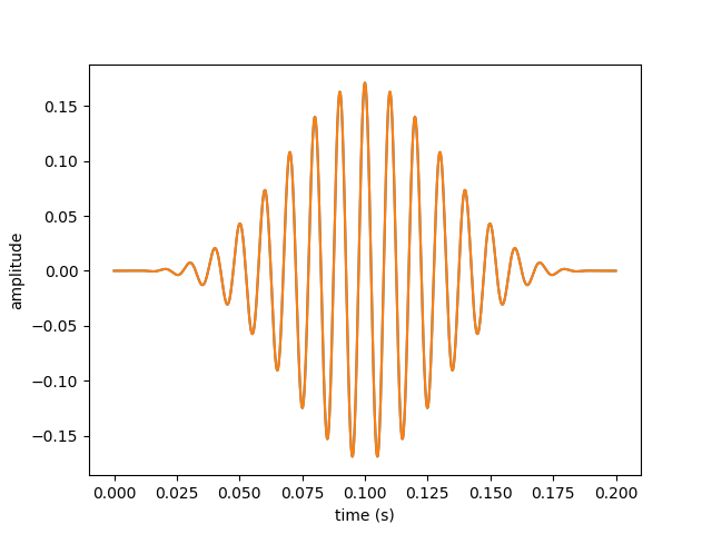
You will note that the frequency is now low enough that the picture can resolve the sine cycles, and we have a Hanning envelope.
Sanity check: do we have the number of sine cycles we expect in the figure?
Comprehension question: the peak amplitude in the second figure is larger, but we did not change the intensity (ABL (dB), that is, the "average binaural level"). The fact that the amplitude changed although the ABL did not - that is not a bug. Do you understand why?
Exercise: try to play with this, make tones of different intensities and frequencies, or different ITDs and ILDs, plot them and listen to them.